Dynamic simulation of a printed circuit board assembly#
This examples shows how to use PyMAPDL to import an existing FE model and to run a modal and PSD analysis. PyDPF modules are also used for post-processing.
The following topics are available:
This example is inspired from the model and analysis defined in Chapter 20 of the Mechanical APDL technology showcase manual.
20.1. Introduction#
20.1.1. Additional packages used#
Matplotlib is used for plotting purposes.
20.1.2. Setting up model#
The original FE model is given in the Ansys Mechanical APDL Technology
showcase manual. The pcb_mesh_file.cdb contains a FE model of a single
circuit board. The model is meshed with SOLID186, SHELL181 and BEAM188 elements.
All components of the PCB model is assigned with linear elastic isotropic materials.
Bonded and flexible surface-to-surface contact pairs are used to define the contact
between the IC packages and the circuit board.
20.1.3. Starting MAPDL as a service#
# sphinx_gallery_thumbnail_path = '_static/tse20_setup.png'

import _.pyplot as plt

from ansys.mapdl.core import launch_mapdl
from ansys.mapdl.core.examples.downloads import download_tech_demo_data

# Start MAPDL as a service
mapdl = launch_mapdl()
print(mapdl)
Product:             Ansys Mechanical Enterprise
MAPDL Version:       21.2
ansys.mapdl Version: 0.63.0
20.2. Modeling#
20.2.1. Importing an external model#
# read model of single circuit board
# download the cdb file
pcb_mesh_file = download_tech_demo_data("td-20", "pcb_mesh_file.cdb")

# Enter preprocessor and read in cdb
mapdl.prep7()
mapdl.cdread("COMB", pcb_mesh_file)
mapdl.allsel()
mapdl.eplot(background="w")
mapdl.cmsel("all")
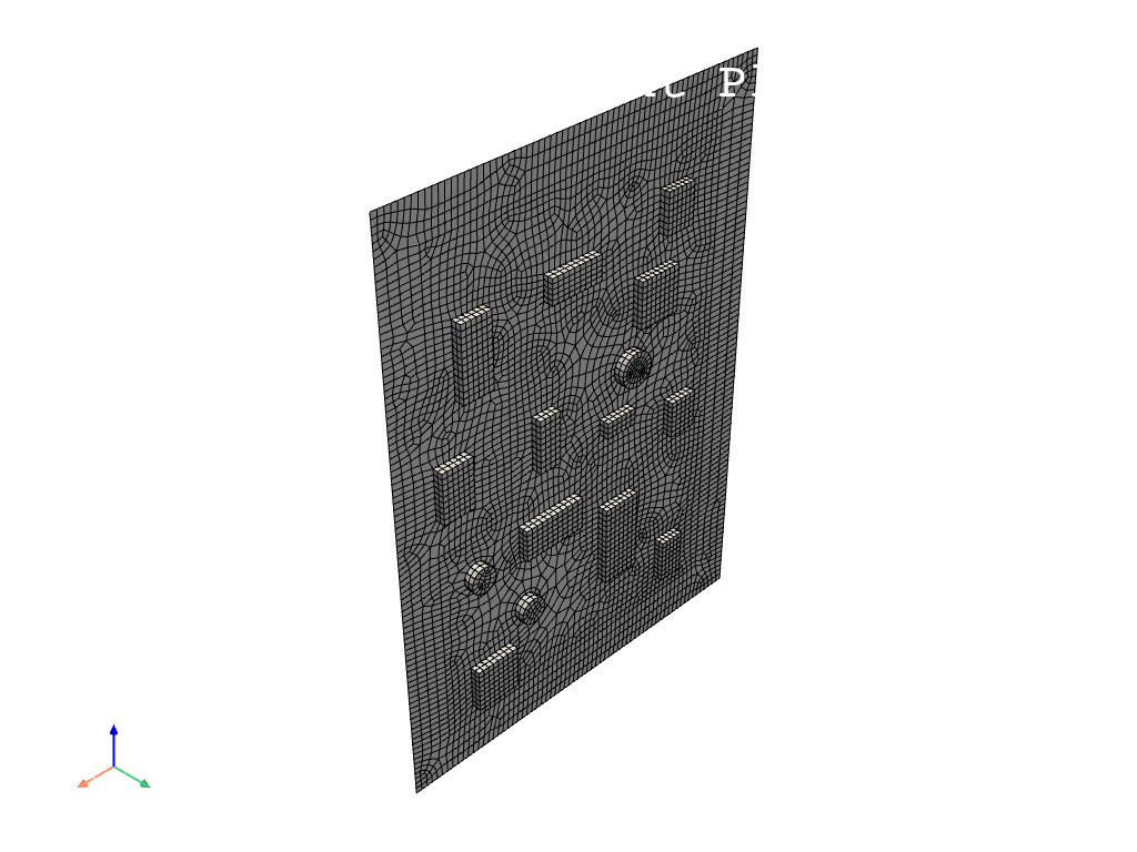
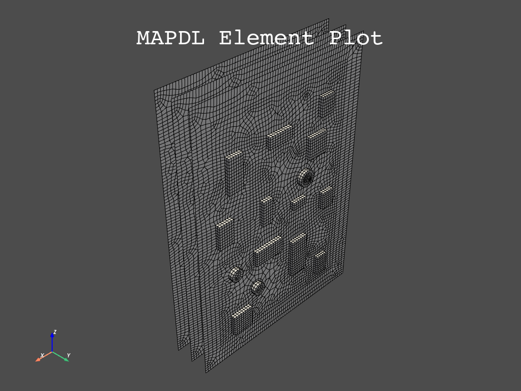
20.2.2. Creating the complete layered model#
The original model will be duplicated to create a layered PCB of three layers that are bound together.
# duplicate single PCB to get three layers
# get the maximum node number for the single layers PCB in the input file
max_nodenum = mapdl.get("max_nodenum", "node", "", "num", "max")

# generate additional PCBs offset by 20 mm in the -y direction
mapdl.egen(3, max_nodenum, "all", dy=-20)


# bind the three layers together
# select components of interest
mapdl.cmsel("s", "N_JOINT_BOARD")
mapdl.cmsel("a", "N_JOINT_LEGS")
mapdl.cmsel("a", "N_BASE")

# get number of currently selected nodes
nb_selected_nodes = mapdl.mesh.n_node
current_node = 0
queries = mapdl.queries

# also select similar nodes for copies of the single PCB
# and couple all dofs at the interface
for node_id in range(1, nb_selected_nodes + 1):
    current_node = queries.ndnext(current_node)
    mapdl.nsel("a", "node", "", current_node + max_nodenum)
    mapdl.nsel("a", "node", "", current_node + 2 * max_nodenum)
mapdl.cpintf("all")

# define fixed support boundary condition
# get max coupled set number
cp_max = mapdl.get("cp_max", "cp", 0, "max")

# unselect nodes scoped in CP equations
mapdl.nsel("u", "cp", "", 1, "cp_max")

# create named selection for base excitation
mapdl.cm("n_base_excite", "node")

# fix displacement for base excitation nodes
mapdl.d("all", "all")

# select all and plot the model using MAPDL's plotter and VTK's
mapdl.allsel("all")
mapdl.cmsel("all")
mapdl.graphics("power")
mapdl.rgb("index", 100, 100, 100, 0)
mapdl.rgb("index", 80, 80, 80, 13)
mapdl.rgb("index", 60, 60, 60, 14)
mapdl.rgb("index", 0, 0, 0, 15)
mapdl.triad("rbot")
mapdl.pnum("type", 1)
mapdl.number(1)
mapdl.hbc(1, "on")
mapdl.pbc("all", "", 1)
mapdl.view(1, 1, 1, 1)
# mapdl.eplot(vtk=False)
mapdl.eplot(vtk=True)
20.3. Modal analysis#
20.3.1. Run modal analysis#
A modal analysis is run using Block Lanczos. Only 10 modes are extracted for the sake of run times, but using a higher number of nodes is recommended (suggestion: 300 modes).
# Enter solution processor and define analysis settings
mapdl.slashsolu()
mapdl.antype("modal")
# set number of modes to extract
# using a higher number of modes is recommended
nb_modes = 10
# use Block Lanczos to extract specified number of modes
mapdl.modopt("lanb", nb_modes)
mapdl.mxpand(nb_modes)
output = mapdl.solve()
print(output)
*** NOTE *** CP = 0.781 TIME= 06:52:51
The automatic domain decomposition logic has selected the MESH domain
decomposition method with 2 processes per solution.
***** ANSYS SOLVE COMMAND *****
*** NOTE *** CP = 0.812 TIME= 06:52:51
There is no title defined for this analysis.
*** NOTE *** CP = 0.828 TIME= 06:52:51
To view 3-D mode shapes of beam or pipe elements, expand the modes with
element results calculation active via the MXPAND command's
Elcalc=YES.
*** WARNING *** CP = 0.844 TIME= 06:52:51
Previous testing revealed that 3 of the 26046 selected elements violate
shape warning limits. To review warning messages, please see the
output or error file, or issue the CHECK command.
*** NOTE *** CP = 0.844 TIME= 06:52:51
The model data was checked and warning messages were found.
Please review output or errors file (
C:\Users\gayuso\AppData\Local\Temp\ansys_pasiuwhdkb\file0.err ) for
these warning messages.
*** SELECTION OF ELEMENT TECHNOLOGIES FOR APPLICABLE ELEMENTS ***
---GIVE SUGGESTIONS ONLY---
ELEMENT TYPE 1 IS BEAM188 . KEYOPT(3) IS ALREADY SET AS SUGGESTED.
ELEMENT TYPE 1 IS BEAM188 . KEYOPT(15) IS ALREADY SET AS SUGGESTED.
ELEMENT TYPE 2 IS BEAM188 . KEYOPT(3) IS ALREADY SET AS SUGGESTED.
ELEMENT TYPE 2 IS BEAM188 . KEYOPT(15) IS ALREADY SET AS SUGGESTED.
ELEMENT TYPE 3 IS BEAM188 . KEYOPT(3) IS ALREADY SET AS SUGGESTED.
ELEMENT TYPE 3 IS BEAM188 . KEYOPT(15) IS ALREADY SET AS SUGGESTED.
ELEMENT TYPE 4 IS BEAM188 . KEYOPT(3) IS ALREADY SET AS SUGGESTED.
ELEMENT TYPE 4 IS BEAM188 . KEYOPT(15) IS ALREADY SET AS SUGGESTED.
ELEMENT TYPE 5 IS BEAM188 . KEYOPT(3) IS ALREADY SET AS SUGGESTED.
ELEMENT TYPE 5 IS BEAM188 . KEYOPT(15) IS ALREADY SET AS SUGGESTED.
ELEMENT TYPE 6 IS SHELL181. IT IS ASSOCIATED WITH ELASTOPLASTIC
MATERIALS ONLY. KEYOPT(8)=2 IS SUGGESTED AND KEYOPT(3)=2 IS SUGGESTED FOR
HIGHER ACCURACY OF MEMBRANE STRESSES; OTHERWISE, KEYOPT(3)=0 IS SUGGESTED.
ELEMENT TYPE 6 HAS KEYOPT(3)=2. FOR THE SPECIFIED ANALYSIS TYPE, LUMPED MASS
MATRIX OPTION (LUMPM, ON) IS SUGGESTED.
ELEMENT TYPE 7 IS SOLID186. KEYOPT(2)=0 IS SUGGESTED.
ELEMENT TYPE 8 IS SOLID186. KEYOPT(2)=0 IS SUGGESTED.
ELEMENT TYPE 9 IS SOLID186. KEYOPT(2)=0 IS SUGGESTED.
ELEMENT TYPE 10 IS SOLID186. KEYOPT(2)=0 IS SUGGESTED.
ELEMENT TYPE 11 IS SOLID186. KEYOPT(2)=0 IS SUGGESTED.
ELEMENT TYPE 12 IS SOLID186. KEYOPT(2)=0 IS SUGGESTED.
ELEMENT TYPE 13 IS SOLID186. KEYOPT(2)=0 IS SUGGESTED.
ELEMENT TYPE 14 IS SOLID186. KEYOPT(2)=0 IS SUGGESTED.
ELEMENT TYPE 15 IS SOLID186. KEYOPT(2)=0 IS SUGGESTED.
ELEMENT TYPE 16 IS SOLID186. KEYOPT(2)=0 IS SUGGESTED.
ELEMENT TYPE 17 IS SOLID186. KEYOPT(2)=0 IS SUGGESTED.
ELEMENT TYPE 18 IS SOLID186. KEYOPT(2)=0 IS SUGGESTED.
ELEMENT TYPE 19 IS SOLID186. KEYOPT(2)=0 IS SUGGESTED.
ELEMENT TYPE 20 IS SOLID186. KEYOPT(2)=0 IS SUGGESTED.
ELEMENT TYPE 21 IS SOLID186. KEYOPT(2)=0 IS SUGGESTED.
*** ANSYS - ENGINEERING ANALYSIS SYSTEM RELEASE 2021 R2 21.2 ***
DISTRIBUTED Ansys Mechanical Enterprise
00000000 VERSION=WINDOWS x64 06:52:51 JUL 25, 2022 CP= 0.844
S O L U T I O N O P T I O N S
PROBLEM DIMENSIONALITY. . . . . . . . . . . . .3-D
DEGREES OF FREEDOM. . . . . . UX UY UZ ROTX ROTY ROTZ
ANALYSIS TYPE . . . . . . . . . . . . . . . . .MODAL
EXTRACTION METHOD. . . . . . . . . . . . . .BLOCK LANCZOS
NUMBER OF MODES TO EXTRACT. . . . . . . . . . . 10
GLOBALLY ASSEMBLED MATRIX . . . . . . . . . . .SYMMETRIC
NUMBER OF MODES TO EXPAND . . . . . . . . . . . 10
ELEMENT RESULTS CALCULATION . . . . . . . . . .OFF
*** NOTE *** CP = 0.844 TIME= 06:52:51
SHELL181 and SHELL281 will not support real constant input at a future
release. Please move to section input.
*** NOTE *** CP = 0.891 TIME= 06:52:51
The conditions for direct assembly have been met. No .emat or .erot
files will be produced.
*** NOTE *** CP = 0.922 TIME= 06:52:51
Internal nodes from 43998 to 44297 are created.
300 internal nodes are used for quadratic and/or cubic options of
BEAM188, PIPE288, and/or SHELL208.
*** NOTE *** CP = 1.953 TIME= 06:52:52
Symmetric Deformable- deformable contact pair identified by real
constant set 22 and contact element type 22 has been set up. The
companion pair has real constant set ID 23. Both pairs should have
the same behavior.
ANSYS will keep the current pair and deactivate its companion pair,
resulting in asymmetric contact.
Shell edge - solid surface constraint is built
Contact algorithm: MPC based approach
*** NOTE *** CP = 1.953 TIME= 06:52:52
Contact related postprocess items (ETABLE, pressure ...) are not
available.
Contact detection at: nodal point (normal to target surface)
MPC will be built internally to handle bonded contact.
Default influence distance FTOLN will be used.
Average contact surface length 3.0609
Average contact pair depth 4.0000
User defined pinball region PINB 0.86250
Default target edge extension factor TOLS 10.000
Initial penetration/gap is excluded.
Bonded contact (always) is defined.
*** NOTE *** CP = 1.953 TIME= 06:52:52
Max. Initial penetration 7.105427358E-15 was detected between contact
element 23362 and target element 23450.
****************************************
*** NOTE *** CP = 1.953 TIME= 06:52:52
Symmetric Deformable- deformable contact pair identified by real
constant set 23 and contact element type 22 has been set up. The
companion pair has real constant set ID 22. Both pairs should have
the same behavior.
ANSYS will deactivate the current pair and keep its companion pair,
resulting in asymmetric contact.
Auto surface constraint is built
Contact algorithm: MPC based approach
*** NOTE *** CP = 1.953 TIME= 06:52:52
Contact related postprocess items (ETABLE, pressure ...) are not
available.
Contact detection at: nodal point (normal to target surface)
MPC will be built internally to handle bonded contact.
Average contact surface length 2.6035
Average contact pair depth 2.5000
User defined pinball region PINB 0.86250
Default target edge extension factor TOLS 10.000
Initial penetration/gap is excluded.
Bonded contact (always) is defined.
*** NOTE *** CP = 1.953 TIME= 06:52:52
Max. Initial penetration 7.105427358E-15 was detected between contact
element 23389 and target element 23348.
****************************************
*** NOTE *** CP = 1.953 TIME= 06:52:52
Symmetric Deformable- deformable contact pair identified by real
constant set 24 and contact element type 24 has been set up. The
companion pair has real constant set ID 25. Both pairs should have
the same behavior.
ANSYS will keep the current pair and deactivate its companion pair,
resulting in asymmetric contact.
Shell edge - solid surface constraint is built
Contact algorithm: MPC based approach
*** NOTE *** CP = 1.953 TIME= 06:52:52
Contact related postprocess items (ETABLE, pressure ...) are not
available.
Contact detection at: nodal point (normal to target surface)
MPC will be built internally to handle bonded contact.
Default influence distance FTOLN will be used.
Average contact surface length 2.7893
Average contact pair depth 4.0000
User defined pinball region PINB 0.86250
Default target edge extension factor TOLS 10.000
Initial penetration/gap is excluded.
Bonded contact (always) is defined.
*** NOTE *** CP = 1.953 TIME= 06:52:52
Max. Initial penetration 1.065814104E-14 was detected between contact
element 23534 and target element 23703.
***************************************
*** NOTE *** CP = 1.953 TIME= 06:52:52
Symmetric Deformable- deformable contact pair identified by real
constant set 25 and contact element type 24 has been set up. The
companion pair has real constant set ID 24. Both pairs should have
the same behavior.
ANSYS will deactivate the current pair and keep its companion pair,
resulting in asymmetric contact.
Auto surface constraint is built
Contact algorithm: MPC based approach
*** NOTE *** CP = 1.953 TIME= 06:52:52
Contact related postprocess items (ETABLE, pressure ...) are not
available.
Contact detection at: nodal point (normal to target surface)
MPC will be built internally to handle bonded contact.
Average contact surface length 2.6670
Average contact pair depth 2.5000
User defined pinball region PINB 0.86250
Default target edge extension factor TOLS 10.000
Initial penetration/gap is excluded.
Bonded contact (always) is defined.
*** NOTE *** CP = 1.953 TIME= 06:52:52
Max. Initial penetration 7.105427358E-15 was detected between contact
element 23619 and target element 23500.
***************************************
*** NOTE *** CP = 1.953 TIME= 06:52:52
Symmetric Deformable- deformable contact pair identified by real
constant set 26 and contact element type 26 has been set up. The
companion pair has real constant set ID 27. Both pairs should have
the same behavior.
ANSYS will keep the current pair and deactivate its companion pair,
resulting in asymmetric contact.
Shell edge - solid surface constraint is built
Contact algorithm: MPC based approach
*** NOTE *** CP = 1.953 TIME= 06:52:52
Contact related postprocess items (ETABLE, pressure ...) are not
available.
Contact detection at: nodal point (normal to target surface)
MPC will be built internally to handle bonded contact.
Default influence distance FTOLN will be used.
Average contact surface length 2.4344
Average contact pair depth 4.0000
User defined pinball region PINB 0.86250
Default target edge extension factor TOLS 10.000
Initial penetration/gap is excluded.
Bonded contact (always) is defined.
*** NOTE *** CP = 1.953 TIME= 06:52:52
Max. Initial penetration 7.105427358E-15 was detected between contact
element 23799 and target element 23840.
***************************************
*** NOTE *** CP = 1.953 TIME= 06:52:52
Symmetric Deformable- deformable contact pair identified by real
constant set 27 and contact element type 26 has been set up. The
companion pair has real constant set ID 26. Both pairs should have
the same behavior.
ANSYS will deactivate the current pair and keep its companion pair,
resulting in asymmetric contact.
Auto surface constraint is built
Contact algorithm: MPC based approach
*** NOTE *** CP = 1.953 TIME= 06:52:52
Contact related postprocess items (ETABLE, pressure ...) are not
available.
Contact detection at: nodal point (normal to target surface)
MPC will be built internally to handle bonded contact.
Average contact surface length 2.2769
Average contact pair depth 2.5000
User defined pinball region PINB 0.86250
Default target edge extension factor TOLS 10.000
Initial penetration/gap is excluded.
Bonded contact (always) is defined.
*** NOTE *** CP = 1.953 TIME= 06:52:52
Max. Initial penetration 8.437694987E-15 was detected between contact
element 23816 and target element 23774.
****************************************
*** NOTE *** CP = 1.953 TIME= 06:52:52
Symmetric Deformable- deformable contact pair identified by real
constant set 28 and contact element type 28 has been set up. The
companion pair has real constant set ID 29. Both pairs should have
the same behavior.
ANSYS will keep the current pair and deactivate its companion pair,
resulting in asymmetric contact.
Shell edge - solid surface constraint is built
Contact algorithm: MPC based approach
*** NOTE *** CP = 1.953 TIME= 06:52:52
Contact related postprocess items (ETABLE, pressure ...) are not
available.
Contact detection at: nodal point (normal to target surface)
MPC will be built internally to handle bonded contact.
Default influence distance FTOLN will be used.
Average contact surface length 3.2044
Average contact pair depth 4.0000
User defined pinball region PINB 0.86250
Default target edge extension factor TOLS 10.000
Initial penetration/gap is excluded.
Bonded contact (always) is defined.
*** NOTE *** CP = 1.953 TIME= 06:52:52
Max. Initial penetration 1.065814104E-14 was detected between contact
element 23925 and target element 24048.
****************************************
*** NOTE *** CP = 1.953 TIME= 06:52:52
Symmetric Deformable- deformable contact pair identified by real
constant set 29 and contact element type 28 has been set up. The
companion pair has real constant set ID 28. Both pairs should have
the same behavior.
ANSYS will deactivate the current pair and keep its companion pair,
resulting in asymmetric contact.
Auto surface constraint is built
Contact algorithm: MPC based approach
*** NOTE *** CP = 1.953 TIME= 06:52:52
Contact related postprocess items (ETABLE, pressure ...) are not
available.
Contact detection at: nodal point (normal to target surface)
MPC will be built internally to handle bonded contact.
Average contact surface length 2.8833
Average contact pair depth 2.5000
User defined pinball region PINB 0.86250
Default target edge extension factor TOLS 10.000
Initial penetration/gap is excluded.
Bonded contact (always) is defined.
*** NOTE *** CP = 1.953 TIME= 06:52:52
Max. Initial penetration 7.993605777E-15 was detected between contact
element 24004 and target element 23917.
****************************************
*** NOTE *** CP = 1.953 TIME= 06:52:52
Symmetric Deformable- deformable contact pair identified by real
constant set 30 and contact element type 30 has been set up. The
companion pair has real constant set ID 31. Both pairs should have
the same behavior.
ANSYS will keep the current pair and deactivate its companion pair,
resulting in asymmetric contact.
Shell edge - solid surface constraint is built
Contact algorithm: MPC based approach
*** NOTE *** CP = 1.953 TIME= 06:52:52
Contact related postprocess items (ETABLE, pressure ...) are not
available.
Contact detection at: nodal point (normal to target surface)
MPC will be built internally to handle bonded contact.
Default influence distance FTOLN will be used.
Average contact surface length 2.6992
Average contact pair depth 4.0000
User defined pinball region PINB 0.86250
Default target edge extension factor TOLS 10.000
Initial penetration/gap is excluded.
Bonded contact (always) is defined.
*** NOTE *** CP = 1.953 TIME= 06:52:52
Max. Initial penetration 1.33226763E-14 was detected between contact
element 24136 and target element 24168.
****************************************
*** NOTE *** CP = 1.953 TIME= 06:52:52
Symmetric Deformable- deformable contact pair identified by real
constant set 31 and contact element type 30 has been set up. The
companion pair has real constant set ID 30. Both pairs should have
the same behavior.
ANSYS will deactivate the current pair and keep its companion pair,
resulting in asymmetric contact.
Auto surface constraint is built
Contact algorithm: MPC based approach
*** NOTE *** CP = 1.953 TIME= 06:52:52
Contact related postprocess items (ETABLE, pressure ...) are not
available.
Contact detection at: nodal point (normal to target surface)
MPC will be built internally to handle bonded contact.
Average contact surface length 2.7212
Average contact pair depth 2.5000
User defined pinball region PINB 0.86250
Default target edge extension factor TOLS 10.000
Initial penetration/gap is excluded.
Bonded contact (always) is defined.
*** NOTE *** CP = 1.953 TIME= 06:52:52
Max. Initial penetration 1.065814104E-14 was detected between contact
element 24143 and target element 24111.
****************************************
*** NOTE *** CP = 1.953 TIME= 06:52:52
Symmetric Deformable- deformable contact pair identified by real
constant set 32 and contact element type 32 has been set up. The
companion pair has real constant set ID 33. Both pairs should have
the same behavior.
ANSYS will keep the current pair and deactivate its companion pair,
resulting in asymmetric contact.
Shell edge - solid surface constraint is built
Contact algorithm: MPC based approach
*** NOTE *** CP = 1.953 TIME= 06:52:52
Contact related postprocess items (ETABLE, pressure ...) are not
available.
Contact detection at: nodal point (normal to target surface)
MPC will be built internally to handle bonded contact.
Default influence distance FTOLN will be used.
Average contact surface length 3.1818
Average contact pair depth 4.0000
User defined pinball region PINB 0.86250
Default target edge extension factor TOLS 10.000
Initial penetration/gap is excluded.
Bonded contact (always) is defined.
*** NOTE *** CP = 1.953 TIME= 06:52:52
Max. Initial penetration 2.131628207E-14 was detected between contact
element 24242 and target element 24365.
****************************************
*** NOTE *** CP = 1.953 TIME= 06:52:52
Symmetric Deformable- deformable contact pair identified by real
constant set 33 and contact element type 32 has been set up. The
companion pair has real constant set ID 32. Both pairs should have
the same behavior.
ANSYS will deactivate the current pair and keep its companion pair,
resulting in asymmetric contact.
Auto surface constraint is built
Contact algorithm: MPC based approach
*** NOTE *** CP = 1.953 TIME= 06:52:52
Contact related postprocess items (ETABLE, pressure ...) are not
available.
Contact detection at: nodal point (normal to target surface)
MPC will be built internally to handle bonded contact.
Average contact surface length 2.7511
Average contact pair depth 2.5000
User defined pinball region PINB 0.86250
Default target edge extension factor TOLS 10.000
Initial penetration/gap is excluded.
Bonded contact (always) is defined.
*** NOTE *** CP = 1.953 TIME= 06:52:52
Max. Initial penetration 7.105427358E-15 was detected between contact
element 24279 and target element 24217.
***************************************
*** NOTE *** CP = 1.953 TIME= 06:52:52
Symmetric Deformable- deformable contact pair identified by real
constant set 34 and contact element type 34 has been set up. The
companion pair has real constant set ID 35. Both pairs should have
the same behavior.
ANSYS will keep the current pair and deactivate its companion pair,
resulting in asymmetric contact.
Shell edge - solid surface constraint is built
Contact algorithm: MPC based approach
*** NOTE *** CP = 1.953 TIME= 06:52:52
Contact related postprocess items (ETABLE, pressure ...) are not
available.
Contact detection at: nodal point (normal to target surface)
MPC will be built internally to handle bonded contact.
Default influence distance FTOLN will be used.
Average contact surface length 3.2093
Average contact pair depth 4.0000
User defined pinball region PINB 0.86250
Default target edge extension factor TOLS 10.000
Initial penetration/gap is excluded.
Bonded contact (always) is defined.
*** NOTE *** CP = 1.953 TIME= 06:52:52
Max. Initial penetration 7.105427358E-15 was detected between contact
element 24457 and target element 24613.
****************************************
*** NOTE *** CP = 1.953 TIME= 06:52:52
Symmetric Deformable- deformable contact pair identified by real
constant set 35 and contact element type 34 has been set up. The
companion pair has real constant set ID 34. Both pairs should have
the same behavior.
ANSYS will deactivate the current pair and keep its companion pair,
resulting in asymmetric contact.
Auto surface constraint is built
Contact algorithm: MPC based approach
*** NOTE *** CP = 1.953 TIME= 06:52:52
Contact related postprocess items (ETABLE, pressure ...) are not
available.
Contact detection at: nodal point (normal to target surface)
MPC will be built internally to handle bonded contact.
Average contact surface length 2.7849
Average contact pair depth 2.5000
User defined pinball region PINB 0.86250
Default target edge extension factor TOLS 10.000
Initial penetration/gap is excluded.
Bonded contact (always) is defined.
*** NOTE *** CP = 1.953 TIME= 06:52:52
Max. Initial penetration 1.065814104E-14 was detected between contact
element 24514 and target element 24456.
****************************************
*** NOTE *** CP = 1.953 TIME= 06:52:52
Symmetric Deformable- deformable contact pair identified by real
constant set 36 and contact element type 36 has been set up. The
companion pair has real constant set ID 37. Both pairs should have
the same behavior.
ANSYS will keep the current pair and deactivate its companion pair,
resulting in asymmetric contact.
Shell edge - solid surface constraint is built
Contact algorithm: MPC based approach
*** NOTE *** CP = 1.953 TIME= 06:52:52
Contact related postprocess items (ETABLE, pressure ...) are not
available.
Contact detection at: nodal point (normal to target surface)
MPC will be built internally to handle bonded contact.
Default influence distance FTOLN will be used.
Average contact surface length 2.8622
Average contact pair depth 4.0000
User defined pinball region PINB 0.86250
Default target edge extension factor TOLS 10.000
Initial penetration/gap is excluded.
Bonded contact (always) is defined.
*** NOTE *** CP = 1.953 TIME= 06:52:52
Max. Initial penetration 1.421085472E-14 was detected between contact
element 24670 and target element 24765.
****************************************
*** NOTE *** CP = 1.953 TIME= 06:52:52
Symmetric Deformable- deformable contact pair identified by real
constant set 37 and contact element type 36 has been set up. The
companion pair has real constant set ID 36. Both pairs should have
the same behavior.
ANSYS will deactivate the current pair and keep its companion pair,
resulting in asymmetric contact.
Auto surface constraint is built
Contact algorithm: MPC based approach
*** NOTE *** CP = 1.953 TIME= 06:52:52
Contact related postprocess items (ETABLE, pressure ...) are not
available.
Contact detection at: nodal point (normal to target surface)
MPC will be built internally to handle bonded contact.
Average contact surface length 2.7993
Average contact pair depth 2.5000
User defined pinball region PINB 0.86250
Default target edge extension factor TOLS 10.000
Initial penetration/gap is excluded.
Bonded contact (always) is defined.
*** NOTE *** CP = 1.953 TIME= 06:52:52
Max. Initial penetration 7.105427358E-15 was detected between contact
element 24705 and target element 24663.
****************************************
*** NOTE *** CP = 1.953 TIME= 06:52:52
Symmetric Deformable- deformable contact pair identified by real
constant set 38 and contact element type 38 has been set up. The
companion pair has real constant set ID 39. Both pairs should have
the same behavior.
ANSYS will keep the current pair and deactivate its companion pair,
resulting in asymmetric contact.
Shell edge - solid surface constraint is built
Contact algorithm: MPC based approach
*** NOTE *** CP = 1.953 TIME= 06:52:52
Contact related postprocess items (ETABLE, pressure ...) are not
available.
Contact detection at: nodal point (normal to target surface)
MPC will be built internally to handle bonded contact.
Default influence distance FTOLN will be used.
Average contact surface length 3.2658
Average contact pair depth 4.0000
User defined pinball region PINB 0.86250
Default target edge extension factor TOLS 10.000
Initial penetration/gap is excluded.
Bonded contact (always) is defined.
*** NOTE *** CP = 1.953 TIME= 06:52:52
Max. Initial penetration 9.769962617E-15 was detected between contact
element 24836 and target element 24926.
****************************************
*** NOTE *** CP = 1.953 TIME= 06:52:52
Symmetric Deformable- deformable contact pair identified by real
constant set 39 and contact element type 38 has been set up. The
companion pair has real constant set ID 38. Both pairs should have
the same behavior.
ANSYS will deactivate the current pair and keep its companion pair,
resulting in asymmetric contact.
Auto surface constraint is built
Contact algorithm: MPC based approach
*** NOTE *** CP = 1.953 TIME= 06:52:52
Contact related postprocess items (ETABLE, pressure ...) are not
available.
Contact detection at: nodal point (normal to target surface)
MPC will be built internally to handle bonded contact.
Average contact surface length 2.8514
Average contact pair depth 2.5000
User defined pinball region PINB 0.86250
Default target edge extension factor TOLS 10.000
Initial penetration/gap is excluded.
Bonded contact (always) is defined.
*** NOTE *** CP = 1.953 TIME= 06:52:52
Max. Initial penetration 8.881784197E-15 was detected between contact
element 24879 and target element 24787.
****************************************
*** NOTE *** CP = 1.953 TIME= 06:52:52
Symmetric Deformable- deformable contact pair identified by real
constant set 40 and contact element type 40 has been set up. The
companion pair has real constant set ID 41. Both pairs should have
the same behavior.
ANSYS will keep the current pair and deactivate its companion pair,
resulting in asymmetric contact.
Shell edge - solid surface constraint is built
Contact algorithm: MPC based approach
*** NOTE *** CP = 1.953 TIME= 06:52:52
Contact related postprocess items (ETABLE, pressure ...) are not
available.
Contact detection at: nodal point (normal to target surface)
MPC will be built internally to handle bonded contact.
Default influence distance FTOLN will be used.
Average contact surface length 2.8593
Average contact pair depth 4.0000
Pinball region factor PINB 1.0000
The resulting pinball region 4.0000
*** NOTE *** CP = 1.953 TIME= 06:52:52
One of the contact searching regions contains at least 63 target
elements. You may reduce the pinball radius.
Default target edge extension factor TOLS 10.000
Initial penetration/gap is excluded.
Bonded contact (always) is defined.
*** NOTE *** CP = 1.953 TIME= 06:52:52
Max. Initial penetration 1.421085472E-14 was detected between contact
element 24979 and target element 25077.
***************************************
*** NOTE *** CP = 1.953 TIME= 06:52:52
Symmetric Deformable- deformable contact pair identified by real
constant set 41 and contact element type 40 has been set up. The
companion pair has real constant set ID 40. Both pairs should have
the same behavior.
ANSYS will deactivate the current pair and keep its companion pair,
resulting in asymmetric contact.
Auto surface constraint is built
Contact algorithm: MPC based approach
*** NOTE *** CP = 1.953 TIME= 06:52:52
Contact related postprocess items (ETABLE, pressure ...) are not
available.
Contact detection at: nodal point (normal to target surface)
MPC will be built internally to handle bonded contact.
Average contact surface length 1.8845
Average contact pair depth 2.5000
Pinball region factor PINB 1.0000
The resulting pinball region 2.5000
Default target edge extension factor TOLS 10.000
Initial penetration/gap is excluded.
Bonded contact (always) is defined.
*** NOTE *** CP = 1.953 TIME= 06:52:52
Max. Initial penetration 1.065814104E-14 was detected between contact
element 25011 and target element 24931.
****************************************
*** NOTE *** CP = 1.953 TIME= 06:52:52
Symmetric Deformable- deformable contact pair identified by real
constant set 42 and contact element type 42 has been set up. The
companion pair has real constant set ID 43. Both pairs should have
the same behavior.
ANSYS will keep the current pair and deactivate its companion pair,
resulting in asymmetric contact.
Shell edge - solid surface constraint is built
Contact algorithm: MPC based approach
*** NOTE *** CP = 1.953 TIME= 06:52:52
Contact related postprocess items (ETABLE, pressure ...) are not
available.
Contact detection at: nodal point (normal to target surface)
MPC will be built internally to handle bonded contact.
Default influence distance FTOLN will be used.
Average contact surface length 2.2391
Average contact pair depth 4.0000
Pinball region factor PINB 1.0000
The resulting pinball region 4.0000
Default target edge extension factor TOLS 10.000
Initial penetration/gap is excluded.
Bonded contact (always) is defined.
*** NOTE *** CP = 1.953 TIME= 06:52:52
Max. Initial penetration 8.881784197E-15 was detected between contact
element 25172 and target element 25232.
***************************************
*** NOTE *** CP = 1.953 TIME= 06:52:52
Symmetric Deformable- deformable contact pair identified by real
constant set 43 and contact element type 42 has been set up. The
companion pair has real constant set ID 42. Both pairs should have
the same behavior.
ANSYS will deactivate the current pair and keep its companion pair,
resulting in asymmetric contact.
Auto surface constraint is built
Contact algorithm: MPC based approach
*** NOTE *** CP = 1.953 TIME= 06:52:52
Contact related postprocess items (ETABLE, pressure ...) are not
available.
Contact detection at: nodal point (normal to target surface)
MPC will be built internally to handle bonded contact.
Average contact surface length 2.4761
Average contact pair depth 2.5000
Pinball region factor PINB 1.0000
The resulting pinball region 2.5000
Default target edge extension factor TOLS 10.000
Initial penetration/gap is excluded.
Bonded contact (always) is defined.
*** NOTE *** CP = 1.953 TIME= 06:52:52
Max. Initial penetration 7.105427358E-15 was detected between contact
element 25184 and target element 25127.
****************************************
*** NOTE *** CP = 1.953 TIME= 06:52:52
Symmetric Deformable- deformable contact pair identified by real
constant set 44 and contact element type 44 has been set up. The
companion pair has real constant set ID 45. Both pairs should have
the same behavior.
ANSYS will keep the current pair and deactivate its companion pair,
resulting in asymmetric contact.
Shell edge - solid surface constraint is built
Contact algorithm: MPC based approach
*** NOTE *** CP = 1.953 TIME= 06:52:52
Contact related postprocess items (ETABLE, pressure ...) are not
available.
Contact detection at: nodal point (normal to target surface)
MPC will be built internally to handle bonded contact.
Default influence distance FTOLN will be used.
Average contact surface length 3.3552
Average contact pair depth 4.0000
User defined pinball region PINB 0.86250
Default target edge extension factor TOLS 10.000
Initial penetration/gap is excluded.
Bonded contact (always) is defined.
*** NOTE *** CP = 1.953 TIME= 06:52:52
Max. Initial penetration 1.421085472E-14 was detected between contact
element 25356 and target element 25570.
****************************************
*** NOTE *** CP = 1.953 TIME= 06:52:52
Symmetric Deformable- deformable contact pair identified by real
constant set 45 and contact element type 44 has been set up. The
companion pair has real constant set ID 44. Both pairs should have
the same behavior.
ANSYS will deactivate the current pair and keep its companion pair,
resulting in asymmetric contact.
Auto surface constraint is built
Contact algorithm: MPC based approach
*** NOTE *** CP = 1.953 TIME= 06:52:52
Contact related postprocess items (ETABLE, pressure ...) are not
available.
Contact detection at: nodal point (normal to target surface)
MPC will be built internally to handle bonded contact.
Average contact surface length 2.7967
Average contact pair depth 2.5000
User defined pinball region PINB 0.86250
Default target edge extension factor TOLS 10.000
Initial penetration/gap is excluded.
Bonded contact (always) is defined.
*** NOTE *** CP = 1.953 TIME= 06:52:52
Max. Initial penetration 1.065814104E-14 was detected between contact
element 25446 and target element 25239.
****************************************
*** NOTE *** CP = 1.953 TIME= 06:52:52
Symmetric Deformable- deformable contact pair identified by real
constant set 46 and contact element type 46 has been set up. The
companion pair has real constant set ID 47. Both pairs should have
the same behavior.
ANSYS will keep the current pair and deactivate its companion pair,
resulting in asymmetric contact.
Shell edge - solid surface constraint is built
Contact algorithm: MPC based approach
*** NOTE *** CP = 1.953 TIME= 06:52:52
Contact related postprocess items (ETABLE, pressure ...) are not
available.
Contact detection at: nodal point (normal to target surface)
MPC will be built internally to handle bonded contact.
Default influence distance FTOLN will be used.
Average contact surface length 3.1237
Average contact pair depth 4.0000
User defined pinball region PINB 0.86250
Default target edge extension factor TOLS 10.000
Initial penetration/gap is excluded.
Bonded contact (always) is defined.
*** NOTE *** CP = 1.953 TIME= 06:52:52
Max. Initial penetration 1.421085472E-14 was detected between contact
element 25628 and target element 25709.
****************************************
*** NOTE *** CP = 1.953 TIME= 06:52:52
Symmetric Deformable- deformable contact pair identified by real
constant set 47 and contact element type 46 has been set up. The
companion pair has real constant set ID 46. Both pairs should have
the same behavior.
ANSYS will deactivate the current pair and keep its companion pair,
resulting in asymmetric contact.
Auto surface constraint is built
Contact algorithm: MPC based approach
*** NOTE *** CP = 1.953 TIME= 06:52:52
Contact related postprocess items (ETABLE, pressure ...) are not
available.
Contact detection at: nodal point (normal to target surface)
MPC will be built internally to handle bonded contact.
Average contact surface length 2.5685
Average contact pair depth 2.5000
User defined pinball region PINB 0.86250
Default target edge extension factor TOLS 10.000
Initial penetration/gap is excluded.
Bonded contact (always) is defined.
*** NOTE *** CP = 1.953 TIME= 06:52:52
Max. Initial penetration 7.105427358E-15 was detected between contact
element 25639 and target element 25608.
****************************************
*** NOTE *** CP = 1.953 TIME= 06:52:52
Symmetric Deformable- deformable contact pair identified by real
constant set 48 and contact element type 48 has been set up. The
companion pair has real constant set ID 49. Both pairs should have
the same behavior.
ANSYS will keep the current pair and deactivate its companion pair,
resulting in asymmetric contact.
Shell edge - solid surface constraint is built
Contact algorithm: MPC based approach
*** NOTE *** CP = 1.953 TIME= 06:52:52
Contact related postprocess items (ETABLE, pressure ...) are not
available.
Contact detection at: nodal point (normal to target surface)
MPC will be built internally to handle bonded contact.
Default influence distance FTOLN will be used.
Average contact surface length 3.0637
Average contact pair depth 4.0000
User defined pinball region PINB 0.86250
Default target edge extension factor TOLS 10.000
Initial penetration/gap is excluded.
Bonded contact (always) is defined.
*** NOTE *** CP = 1.953 TIME= 06:52:52
Max. Initial penetration 1.421085472E-14 was detected between contact
element 25779 and target element 25820.
****************************************
*** NOTE *** CP = 1.953 TIME= 06:52:52
Symmetric Deformable- deformable contact pair identified by real
constant set 49 and contact element type 48 has been set up. The
companion pair has real constant set ID 48. Both pairs should have
the same behavior.
ANSYS will deactivate the current pair and keep its companion pair,
resulting in asymmetric contact.
Auto surface constraint is built
Contact algorithm: MPC based approach
*** NOTE *** CP = 1.953 TIME= 06:52:52
Contact related postprocess items (ETABLE, pressure ...) are not
available.
Contact detection at: nodal point (normal to target surface)
MPC will be built internally to handle bonded contact.
Average contact surface length 2.8027
Average contact pair depth 2.5000
User defined pinball region PINB 0.86250
Default target edge extension factor TOLS 10.000
Initial penetration/gap is excluded.
Bonded contact (always) is defined.
*** NOTE *** CP = 1.953 TIME= 06:52:52
Max. Initial penetration 1.421085472E-14 was detected between contact
element 25787 and target element 25736.
****************************************
*** NOTE *** CP = 1.953 TIME= 06:52:52
Symmetric Deformable- deformable contact pair identified by real
constant set 50 and contact element type 50 has been set up. The
companion pair has real constant set ID 51. Both pairs should have
the same behavior.
ANSYS will keep the current pair and deactivate its companion pair,
resulting in asymmetric contact.
Shell edge - solid surface constraint is built
Contact algorithm: MPC based approach
*** NOTE *** CP = 1.953 TIME= 06:52:52
Contact related postprocess items (ETABLE, pressure ...) are not
available.
Contact detection at: nodal point (normal to target surface)
MPC will be built internally to handle bonded contact.
Default influence distance FTOLN will be used.
Average contact surface length 3.2471
Average contact pair depth 4.0000
User defined pinball region PINB 0.86250
Default target edge extension factor TOLS 10.000
Initial penetration/gap is excluded.
Bonded contact (always) is defined.
*** NOTE *** CP = 1.953 TIME= 06:52:52
Max. Initial penetration 1.33226763E-14 was detected between contact
element 25924 and target element 26035.
****************************************
*** NOTE *** CP = 1.953 TIME= 06:52:52
Symmetric Deformable- deformable contact pair identified by real
constant set 51 and contact element type 50 has been set up. The
companion pair has real constant set ID 50. Both pairs should have
the same behavior.
ANSYS will deactivate the current pair and keep its companion pair,
resulting in asymmetric contact.
Auto surface constraint is built
Contact algorithm: MPC based approach
*** NOTE *** CP = 1.953 TIME= 06:52:52
Contact related postprocess items (ETABLE, pressure ...) are not
available.
Contact detection at: nodal point (normal to target surface)
MPC will be built internally to handle bonded contact.
Average contact surface length 2.6964
Average contact pair depth 2.5000
User defined pinball region PINB 0.86250
Default target edge extension factor TOLS 10.000
Initial penetration/gap is excluded.
Bonded contact (always) is defined.
*** NOTE *** CP = 1.953 TIME= 06:52:52
Max. Initial penetration 7.105427358E-15 was detected between contact
element 25939 and target element 25890.
****************************************
*** NOTE *** CP = 2.016 TIME= 06:52:52
Internal nodes from 43998 to 44297 are created.
300 internal nodes are used for quadratic and/or cubic options of
BEAM188, PIPE288, and/or SHELL208.
D I S T R I B U T E D D O M A I N D E C O M P O S E R
...Number of elements: 26046
...Number of nodes: 44197
...Decompose to 2 CPU domains
...Element load balance ratio = 1.001
L O A D S T E P O P T I O N S
LOAD STEP NUMBER. . . . . . . . . . . . . . . . 1
THERMAL STRAINS INCLUDED IN THE LOAD VECTOR . . YES
PRINT OUTPUT CONTROLS . . . . . . . . . . . . .NO PRINTOUT
DATABASE OUTPUT CONTROLS. . . . . . . . . . . .ALL DATA WRITTEN
*** NOTE *** CP = 2.891 TIME= 06:52:53
Symmetric Deformable- deformable contact pair identified by real
constant set 22 and contact element type 22 has been set up. The
companion pair has real constant set ID 23. Both pairs should have
the same behavior.
ANSYS will keep the current pair and deactivate its companion pair,
resulting in asymmetric contact.
Shell edge - solid surface constraint is built
Contact algorithm: MPC based approach
*** NOTE *** CP = 2.891 TIME= 06:52:53
Contact related postprocess items (ETABLE, pressure ...) are not
available.
Contact detection at: nodal point (normal to target surface)
MPC will be built internally to handle bonded contact.
Default influence distance FTOLN will be used.
Average contact surface length 3.0609
Average contact pair depth 4.0000
User defined pinball region PINB 0.86250
Default target edge extension factor TOLS 10.000
Initial penetration/gap is excluded.
Bonded contact (always) is defined.
*** NOTE *** CP = 2.891 TIME= 06:52:53
Max. Initial penetration 7.105427358E-15 was detected between contact
element 23362 and target element 23450.
****************************************
*** NOTE *** CP = 2.891 TIME= 06:52:53
Symmetric Deformable- deformable contact pair identified by real
constant set 23 and contact element type 22 has been set up. The
companion pair has real constant set ID 22. Both pairs should have
the same behavior.
ANSYS will deactivate the current pair and keep its companion pair,
resulting in asymmetric contact.
Auto surface constraint is built
Contact algorithm: MPC based approach
*** NOTE *** CP = 2.891 TIME= 06:52:53
Contact related postprocess items (ETABLE, pressure ...) are not
available.
Contact detection at: nodal point (normal to target surface)
MPC will be built internally to handle bonded contact.
Average contact surface length 2.6035
Average contact pair depth 2.5000
User defined pinball region PINB 0.86250
Default target edge extension factor TOLS 10.000
Initial penetration/gap is excluded.
Bonded contact (always) is defined.
*** NOTE *** CP = 2.891 TIME= 06:52:53
Max. Initial penetration 7.105427358E-15 was detected between contact
element 23389 and target element 23348.
****************************************
*** NOTE *** CP = 2.891 TIME= 06:52:53
Symmetric Deformable- deformable contact pair identified by real
constant set 24 and contact element type 24 has been set up. The
companion pair has real constant set ID 25. Both pairs should have
the same behavior.
ANSYS will keep the current pair and deactivate its companion pair,
resulting in asymmetric contact.
Shell edge - solid surface constraint is built
Contact algorithm: MPC based approach
*** NOTE *** CP = 2.891 TIME= 06:52:53
Contact related postprocess items (ETABLE, pressure ...) are not
available.
Contact detection at: nodal point (normal to target surface)
MPC will be built internally to handle bonded contact.
Default influence distance FTOLN will be used.
Average contact surface length 2.7893
Average contact pair depth 4.0000
User defined pinball region PINB 0.86250
Default target edge extension factor TOLS 10.000
Initial penetration/gap is excluded.
Bonded contact (always) is defined.
*** NOTE *** CP = 2.891 TIME= 06:52:53
Max. Initial penetration 1.065814104E-14 was detected between contact
element 23534 and target element 23703.
****************************************
*** NOTE *** CP = 2.891 TIME= 06:52:53
Symmetric Deformable- deformable contact pair identified by real
constant set 25 and contact element type 24 has been set up. The
companion pair has real constant set ID 24. Both pairs should have
the same behavior.
ANSYS will deactivate the current pair and keep its companion pair,
resulting in asymmetric contact.
Auto surface constraint is built
Contact algorithm: MPC based approach
*** NOTE *** CP = 2.891 TIME= 06:52:53
Contact related postprocess items (ETABLE, pressure ...) are not
available.
Contact detection at: nodal point (normal to target surface)
MPC will be built internally to handle bonded contact.
Average contact surface length 2.6670
Average contact pair depth 2.5000
User defined pinball region PINB 0.86250
Default target edge extension factor TOLS 10.000
Initial penetration/gap is excluded.
Bonded contact (always) is defined.
*** NOTE *** CP = 2.891 TIME= 06:52:53
Max. Initial penetration 7.105427358E-15 was detected between contact
element 23619 and target element 23500.
****************************************
*** NOTE *** CP = 2.891 TIME= 06:52:53
Symmetric Deformable- deformable contact pair identified by real
constant set 32 and contact element type 32 has been set up. The
companion pair has real constant set ID 33. Both pairs should have
the same behavior.
ANSYS will keep the current pair and deactivate its companion pair,
resulting in asymmetric contact.
Shell edge - solid surface constraint is built
Contact algorithm: MPC based approach
*** NOTE *** CP = 2.891 TIME= 06:52:53
Contact related postprocess items (ETABLE, pressure ...) are not
available.
Contact detection at: nodal point (normal to target surface)
MPC will be built internally to handle bonded contact.
Default influence distance FTOLN will be used.
Average contact surface length 3.1818
Average contact pair depth 4.0000
User defined pinball region PINB 0.86250
Default target edge extension factor TOLS 10.000
Initial penetration/gap is excluded.
Bonded contact (always) is defined.
*** NOTE *** CP = 2.891 TIME= 06:52:53
Max. Initial penetration 2.131628207E-14 was detected between contact
element 24242 and target element 24365.
****************************************
*** NOTE *** CP = 2.891 TIME= 06:52:53
Symmetric Deformable- deformable contact pair identified by real
constant set 33 and contact element type 32 has been set up. The
companion pair has real constant set ID 32. Both pairs should have
the same behavior.
ANSYS will deactivate the current pair and keep its companion pair,
resulting in asymmetric contact.
Auto surface constraint is built
Contact algorithm: MPC based approach
*** NOTE *** CP = 2.891 TIME= 06:52:53
Contact related postprocess items (ETABLE, pressure ...) are not
available.
Contact detection at: nodal point (normal to target surface)
MPC will be built internally to handle bonded contact.
Average contact surface length 2.7511
Average contact pair depth 2.5000
User defined pinball region PINB 0.86250
Default target edge extension factor TOLS 10.000
Initial penetration/gap is excluded.
Bonded contact (always) is defined.
*** NOTE *** CP = 2.891 TIME= 06:52:53
Max. Initial penetration 7.105427358E-15 was detected between contact
element 24279 and target element 24217.
****************************************
*** NOTE *** CP = 2.891 TIME= 06:52:53
Symmetric Deformable- deformable contact pair identified by real
constant set 38 and contact element type 38 has been set up. The
companion pair has real constant set ID 39. Both pairs should have
the same behavior.
ANSYS will keep the current pair and deactivate its companion pair,
resulting in asymmetric contact.
Shell edge - solid surface constraint is built
Contact algorithm: MPC based approach
*** NOTE *** CP = 2.891 TIME= 06:52:53
Contact related postprocess items (ETABLE, pressure ...) are not
available.
Contact detection at: nodal point (normal to target surface)
MPC will be built internally to handle bonded contact.
Default influence distance FTOLN will be used.
Average contact surface length 3.2658
Average contact pair depth 4.0000
User defined pinball region PINB 0.86250
Default target edge extension factor TOLS 10.000
Initial penetration/gap is excluded.
Bonded contact (always) is defined.
*** NOTE *** CP = 2.891 TIME= 06:52:53
Max. Initial penetration 9.769962617E-15 was detected between contact
element 24836 and target element 24926.
****************************************
*** NOTE *** CP = 2.891 TIME= 06:52:53
Symmetric Deformable- deformable contact pair identified by real
constant set 39 and contact element type 38 has been set up. The
companion pair has real constant set ID 38. Both pairs should have
the same behavior.
ANSYS will deactivate the current pair and keep its companion pair,
resulting in asymmetric contact.
Auto surface constraint is built
Contact algorithm: MPC based approach
*** NOTE *** CP = 2.891 TIME= 06:52:53
Contact related postprocess items (ETABLE, pressure ...) are not
available.
Contact detection at: nodal point (normal to target surface)
MPC will be built internally to handle bonded contact.
Average contact surface length 2.8514
Average contact pair depth 2.5000
User defined pinball region PINB 0.86250
Default target edge extension factor TOLS 10.000
Initial penetration/gap is excluded.
Bonded contact (always) is defined.
*** NOTE *** CP = 2.891 TIME= 06:52:53
Max. Initial penetration 8.881784197E-15 was detected between contact
element 24879 and target element 24787.
****************************************
*** NOTE *** CP = 2.891 TIME= 06:52:53
Symmetric Deformable- deformable contact pair identified by real
constant set 40 and contact element type 40 has been set up. The
companion pair has real constant set ID 41. Both pairs should have
the same behavior.
ANSYS will keep the current pair and deactivate its companion pair,
resulting in asymmetric contact.
Shell edge - solid surface constraint is built
Contact algorithm: MPC based approach
*** NOTE *** CP = 2.891 TIME= 06:52:53
Contact related postprocess items (ETABLE, pressure ...) are not
available.
Contact detection at: nodal point (normal to target surface)
MPC will be built internally to handle bonded contact.
Default influence distance FTOLN will be used.
Average contact surface length 2.8593
Average contact pair depth 4.0000
Pinball region factor PINB 1.0000
The resulting pinball region 4.0000
*** NOTE *** CP = 2.891 TIME= 06:52:53
One of the contact searching regions contains at least 63 target
elements. You may reduce the pinball radius.
Default target edge extension factor TOLS 10.000
Initial penetration/gap is excluded.
Bonded contact (always) is defined.
*** NOTE *** CP = 2.891 TIME= 06:52:53
Max. Initial penetration 1.421085472E-14 was detected between contact
element 24979 and target element 25077.
****************************************
*** NOTE *** CP = 2.891 TIME= 06:52:53
Symmetric Deformable- deformable contact pair identified by real
constant set 41 and contact element type 40 has been set up. The
companion pair has real constant set ID 40. Both pairs should have
the same behavior.
ANSYS will deactivate the current pair and keep its companion pair,
resulting in asymmetric contact.
Auto surface constraint is built
Contact algorithm: MPC based approach
*** NOTE *** CP = 2.891 TIME= 06:52:53
Contact related postprocess items (ETABLE, pressure ...) are not
available.
Contact detection at: nodal point (normal to target surface)
MPC will be built internally to handle bonded contact.
Average contact surface length 1.8845
Average contact pair depth 2.5000
Pinball region factor PINB 1.0000
The resulting pinball region 2.5000
Default target edge extension factor TOLS 10.000
Initial penetration/gap is excluded.
Bonded contact (always) is defined.
*** NOTE *** CP = 2.891 TIME= 06:52:53
Max. Initial penetration 1.065814104E-14 was detected between contact
element 25011 and target element 24931.
****************************************
*** NOTE *** CP = 2.891 TIME= 06:52:53
Symmetric Deformable- deformable contact pair identified by real
constant set 48 and contact element type 48 has been set up. The
companion pair has real constant set ID 49. Both pairs should have
the same behavior.
ANSYS will keep the current pair and deactivate its companion pair,
resulting in asymmetric contact.
Shell edge - solid surface constraint is built
Contact algorithm: MPC based approach
*** NOTE *** CP = 2.891 TIME= 06:52:53
Contact related postprocess items (ETABLE, pressure ...) are not
available.
Contact detection at: nodal point (normal to target surface)
MPC will be built internally to handle bonded contact.
Default influence distance FTOLN will be used.
Average contact surface length 3.0637
Average contact pair depth 4.0000
User defined pinball region PINB 0.86250
Default target edge extension factor TOLS 10.000
Initial penetration/gap is excluded.
Bonded contact (always) is defined.
*** NOTE *** CP = 2.891 TIME= 06:52:53
Max. Initial penetration 1.421085472E-14 was detected between contact
element 25779 and target element 25820.
****************************************
*** NOTE *** CP = 2.891 TIME= 06:52:53
Symmetric Deformable- deformable contact pair identified by real
constant set 49 and contact element type 48 has been set up. The
companion pair has real constant set ID 48. Both pairs should have
the same behavior.
ANSYS will deactivate the current pair and keep its companion pair,
resulting in asymmetric contact.
Auto surface constraint is built
Contact algorithm: MPC based approach
*** NOTE *** CP = 2.891 TIME= 06:52:53
Contact related postprocess items (ETABLE, pressure ...) are not
available.
Contact detection at: nodal point (normal to target surface)
MPC will be built internally to handle bonded contact.
Average contact surface length 2.8027
Average contact pair depth 2.5000
User defined pinball region PINB 0.86250
Default target edge extension factor TOLS 10.000
Initial penetration/gap is excluded.
Bonded contact (always) is defined.
*** NOTE *** CP = 2.891 TIME= 06:52:53
Max. Initial penetration 1.421085472E-14 was detected between contact
element 25787 and target element 25736.
****************************************
*** NOTE *** CP = 2.891 TIME= 06:52:53
Symmetric Deformable- deformable contact pair identified by real
constant set 50 and contact element type 50 has been set up. The
companion pair has real constant set ID 51. Both pairs should have
the same behavior.
ANSYS will keep the current pair and deactivate its companion pair,
resulting in asymmetric contact.
Shell edge - solid surface constraint is built
Contact algorithm: MPC based approach
*** NOTE *** CP = 2.891 TIME= 06:52:53
Contact related postprocess items (ETABLE, pressure ...) are not
available.
Contact detection at: nodal point (normal to target surface)
MPC will be built internally to handle bonded contact.
Default influence distance FTOLN will be used.
Average contact surface length 3.2471
Average contact pair depth 4.0000
User defined pinball region PINB 0.86250
Default target edge extension factor TOLS 10.000
Initial penetration/gap is excluded.
Bonded contact (always) is defined.
*** NOTE *** CP = 2.891 TIME= 06:52:53
Max. Initial penetration 1.33226763E-14 was detected between contact
element 25924 and target element 26035.
****************************************
*** NOTE *** CP = 2.891 TIME= 06:52:53
Symmetric Deformable- deformable contact pair identified by real
constant set 51 and contact element type 50 has been set up. The
companion pair has real constant set ID 50. Both pairs should have
the same behavior.
ANSYS will deactivate the current pair and keep its companion pair,
resulting in asymmetric contact.
Auto surface constraint is built
Contact algorithm: MPC based approach
*** NOTE *** CP = 2.891 TIME= 06:52:53
Contact related postprocess items (ETABLE, pressure ...) are not
available.
Contact detection at: nodal point (normal to target surface)
MPC will be built internally to handle bonded contact.
Average contact surface length 2.6964
Average contact pair depth 2.5000
User defined pinball region PINB 0.86250
Default target edge extension factor TOLS 10.000
Initial penetration/gap is excluded.
Bonded contact (always) is defined.
*** NOTE *** CP = 2.891 TIME= 06:52:53
Max. Initial penetration 7.105427358E-15 was detected between contact
element 25939 and target element 25890.
****************************************
*********** PRECISE MASS SUMMARY ***********
TOTAL RIGID BODY MASS MATRIX ABOUT ORIGIN
Translational mass | Coupled translational/rotational mass
0.25166E-03 0.0000 0.0000 | 0.0000 0.34581E-01 0.50068E-02
0.0000 0.25166E-03 0.0000 | -0.34581E-01 0.0000 0.25711E-01
0.0000 0.0000 0.25166E-03 | -0.50068E-02 -0.25711E-01 0.0000
------------------------------------------ | ------------------------------------------
| Rotational mass (inertia)
| 6.4515 0.51185 -3.5215
| 0.51185 9.6801 0.68875
| -3.5215 0.68875 3.5678
TOTAL MASS = 0.25166E-03
The mass principal axes coincide with the global Cartesian axes
CENTER OF MASS (X,Y,Z)= 102.17 -19.895 137.41
TOTAL INERTIA ABOUT CENTER OF MASS
1.5999 0.32438E-03 0.11573E-01
0.32438E-03 2.3014 0.74412E-03
0.11573E-01 0.74412E-03 0.84133
PRINCIPAL INERTIAS = 1.6001 2.3014 0.84115
ORIENTATION VECTORS OF THE INERTIA PRINCIPAL AXES IN GLOBAL CARTESIAN
( 1.000,-0.000, 0.015) ( 0.000, 1.000, 0.001) (-0.015,-0.001, 1.000)
*** MASS SUMMARY BY ELEMENT TYPE ***
TYPE MASS
1 0.326079E-05
2 0.326079E-05
3 0.326079E-05
4 0.326079E-05
5 0.326079E-05
6 0.159600E-03
7 0.429027E-05
8 0.777647E-05
9 0.197978E-05
10 0.735761E-05
11 0.186775E-05
12 0.704400E-05
13 0.696150E-05
14 0.368481E-05
15 0.459882E-05
16 0.330798E-05
17 0.197978E-05
18 0.111823E-04
19 0.391721E-05
20 0.411780E-05
21 0.568872E-05
Range of element maximum matrix coefficients in global coordinates
Maximum = 11792803.9 at element 17387.
Minimum = 528.07874 at element 3660.
*** ELEMENT MATRIX FORMULATION TIMES
TYPE NUMBER ENAME TOTAL CP AVE CP
1 60 BEAM188 0.000 0.000000
2 60 BEAM188 0.000 0.000000
3 60 BEAM188 0.000 0.000000
4 60 BEAM188 0.000 0.000000
5 60 BEAM188 0.000 0.000000
6 13038 SHELL181 1.125 0.000086
7 252 SOLID186 0.062 0.000248
8 432 SOLID186 0.078 0.000181
9 168 SOLID186 0.031 0.000186
10 396 SOLID186 0.000 0.000000
11 108 SOLID186 0.000 0.000000
12 384 SOLID186 0.062 0.000163
13 384 SOLID186 0.016 0.000041
14 210 SOLID186 0.016 0.000074
15 270 SOLID186 0.078 0.000289
16 408 SOLID186 0.047 0.000115
17 150 SOLID186 0.000 0.000000
18 588 SOLID186 0.094 0.000159
19 240 SOLID186 0.078 0.000326
20 216 SOLID186 0.062 0.000289
21 324 SOLID186 0.016 0.000048
22 228 CONTA174 0.016 0.000069
23 228 TARGE170 0.000 0.000000
24 435 CONTA174 0.031 0.000072
25 435 TARGE170 0.000 0.000000
26 156 CONTA174 0.000 0.000000
27 156 TARGE170 0.000 0.000000
28 354 CONTA174 0.000 0.000000
29 354 TARGE170 0.000 0.000000
30 108 CONTA174 0.000 0.000000
31 108 TARGE170 0.000 0.000000
32 348 CONTA174 0.016 0.000045
33 348 TARGE170 0.000 0.000000
34 342 CONTA174 0.000 0.000000
35 342 TARGE170 0.000 0.000000
36 204 CONTA174 0.016 0.000077
37 204 TARGE170 0.000 0.000000
38 234 CONTA174 0.000 0.000000
39 234 TARGE170 0.000 0.000000
40 300 CONTA174 0.047 0.000156
41 300 TARGE170 0.000 0.000000
42 159 CONTA174 0.047 0.000295
43 159 TARGE170 0.000 0.000000
44 519 CONTA174 0.016 0.000030
45 519 TARGE170 0.000 0.000000
46 210 CONTA174 0.000 0.000000
47 210 TARGE170 0.000 0.000000
48 204 CONTA174 0.000 0.000000
49 204 TARGE170 0.000 0.000000
50 288 CONTA174 0.000 0.000000
51 288 TARGE170 0.000 0.000000
Time at end of element matrix formulation CP = 4.40625.
BLOCK LANCZOS CALCULATION OF UP TO 10 EIGENVECTORS.
NUMBER OF EQUATIONS = 159678
MAXIMUM WAVEFRONT = 708
MAXIMUM MODES STORED = 10
MINIMUM EIGENVALUE = 0.00000E+00
MAXIMUM EIGENVALUE = 0.10000E+31
*** NOTE *** CP = 7.078 TIME= 06:52:58
The initial memory allocation (-m) has been exceeded.
Supplemental memory allocations are being used.
Local memory allocated for solver = 470.292 MB
Local memory required for in-core solution = 448.291 MB
Local memory required for out-of-core solution = 208.135 MB
Total memory allocated for solver = 851.493 MB
Total memory required for in-core solution = 811.685 MB
Total memory required for out-of-core solution = 378.173 MB
*** NOTE *** CP = 8.641 TIME= 06:53:00
The Distributed Sparse Matrix Solver used by the Block Lanczos
eigensolver is currently running in the in-core memory mode. This
memory mode uses the most amount of memory in order to avoid using the
hard drive as much as possible, which most often results in the
fastest solution time. This mode is recommended if enough physical
memory is present to accommodate all of the solver data.
*** ANSYS - ENGINEERING ANALYSIS SYSTEM RELEASE 2021 R2 21.2 ***
DISTRIBUTED Ansys Mechanical Enterprise
00000000 VERSION=WINDOWS x64 06:53:02 JUL 25, 2022 CP= 10.781
*** FREQUENCIES FROM BLOCK LANCZOS ITERATION ***
MODE FREQUENCY (HERTZ)
1 21.68428280230
2 21.69024198077
3 21.69131650666
4 33.82973502589
5 33.83798485758
6 33.83938717337
7 37.06064330146
8 37.07091158772
9 37.07187102168
10 43.83753554036
*** ANSYS - ENGINEERING ANALYSIS SYSTEM RELEASE 2021 R2 21.2 ***
DISTRIBUTED Ansys Mechanical Enterprise
00000000 VERSION=WINDOWS x64 06:53:03 JUL 25, 2022 CP= 10.875
***** PARTICIPATION FACTOR CALCULATION ***** X DIRECTION
CUMULATIVE RATIO EFF.MASS
MODE FREQUENCY PERIOD PARTIC.FACTOR RATIO EFFECTIVE MASS MASS FRACTION TO TOTAL MASS
1 21.6843 0.46116E-01 0.13337E-03 1.000000 0.177881E-07 0.312579 0.706832E-04
2 21.6902 0.46104E-01 0.58730E-04 0.440351 0.344927E-08 0.373191 0.137061E-04
3 21.6913 0.46101E-01 0.87053E-04 0.652706 0.757817E-08 0.506358 0.301129E-04
4 33.8297 0.29560E-01 -0.85976E-04 0.644632 0.739184E-08 0.636250 0.293725E-04
5 33.8380 0.29553E-01 -0.38997E-04 0.292392 0.152076E-08 0.662973 0.604293E-05
6 33.8394 0.29551E-01 -0.57555E-04 0.431539 0.331259E-08 0.721184 0.131630E-04
7 37.0606 0.26983E-01 0.25886E-04 0.194086 0.670065E-09 0.732958 0.266259E-05
8 37.0709 0.26975E-01 0.14838E-04 0.111256 0.220178E-09 0.736827 0.874909E-06
9 37.0719 0.26975E-01 0.18637E-04 0.139738 0.347343E-09 0.742931 0.138021E-05
10 43.8375 0.22812E-01 -0.12095E-03 0.906870 0.146291E-07 1.00000 0.581308E-04
-----------------------------------------------------------------------------------------------------------------
sum 0.569074E-07 0.226129E-03
-----------------------------------------------------------------------------------------------------------------
***** PARTICIPATION FACTOR CALCULATION ***** Y DIRECTION
CUMULATIVE RATIO EFF.MASS
MODE FREQUENCY PERIOD PARTIC.FACTOR RATIO EFFECTIVE MASS MASS FRACTION TO TOTAL MASS
1 21.6843 0.46116E-01 0.73666E-02 1.000000 0.542664E-04 0.343547 0.215635
2 21.6902 0.46104E-01 0.33431E-02 0.453826 0.111766E-04 0.414303 0.444117E-01
3 21.6913 0.46101E-01 0.50476E-02 0.685209 0.254787E-04 0.575602 0.101243
4 33.8297 0.29560E-01 0.18755E-02 0.254589 0.351732E-05 0.597869 0.139765E-01
5 33.8380 0.29553E-01 0.89959E-03 0.122118 0.809258E-06 0.602992 0.321569E-02
6 33.8394 0.29551E-01 0.13665E-02 0.185497 0.186726E-05 0.614814 0.741981E-02
7 37.0606 0.26983E-01 0.31196E-02 0.423480 0.973187E-05 0.676423 0.386709E-01
8 37.0709 0.26975E-01 0.19657E-02 0.266836 0.386383E-05 0.700884 0.153535E-01
9 37.0719 0.26975E-01 0.28496E-02 0.386823 0.811999E-05 0.752290 0.322659E-01
10 43.8375 0.22812E-01 0.62552E-02 0.849139 0.391281E-04 1.00000 0.155481
-----------------------------------------------------------------------------------------------------------------
sum 0.157959E-03 0.627673
-----------------------------------------------------------------------------------------------------------------
***** PARTICIPATION FACTOR CALCULATION ***** Z DIRECTION
CUMULATIVE RATIO EFF.MASS
MODE FREQUENCY PERIOD PARTIC.FACTOR RATIO EFFECTIVE MASS MASS FRACTION TO TOTAL MASS
1 21.6843 0.46116E-01 -0.19752E-05 0.023957 0.390136E-11 0.276278E-03 0.155026E-07
2 21.6902 0.46104E-01 -0.13045E-05 0.015822 0.170176E-11 0.396790E-03 0.676218E-08
3 21.6913 0.46101E-01 -0.25987E-05 0.031519 0.675314E-11 0.875019E-03 0.268345E-07
4 33.8297 0.29560E-01 -0.60916E-04 0.738845 0.371071E-08 0.263652 0.147450E-04
5 33.8380 0.29553E-01 -0.30181E-04 0.366070 0.910916E-09 0.328160 0.361965E-05
6 33.8394 0.29551E-01 -0.49330E-04 0.598325 0.243346E-08 0.500487 0.966969E-05
7 37.0606 0.26983E-01 0.12143E-04 0.147286 0.147459E-09 0.510930 0.585948E-06
8 37.0709 0.26975E-01 0.67274E-05 0.081597 0.452579E-10 0.514135 0.179838E-06
9 37.0719 0.26975E-01 0.79651E-05 0.096609 0.634435E-10 0.518628 0.252101E-06
10 43.8375 0.22812E-01 0.82447E-04 1.000000 0.679752E-08 1.00000 0.270109E-04
-----------------------------------------------------------------------------------------------------------------
sum 0.141211E-07 0.561122E-04
-----------------------------------------------------------------------------------------------------------------
***** PARTICIPATION FACTOR CALCULATION *****ROTX DIRECTION
CUMULATIVE RATIO EFF.MASS
MODE FREQUENCY PERIOD PARTIC.FACTOR RATIO EFFECTIVE MASS MASS FRACTION TO TOTAL MASS
1 21.6843 0.46116E-01 -1.0941 1.000000 1.19712 0.282791 0.185559
2 21.6902 0.46104E-01 -0.49643 0.453718 0.246440 0.341006 0.381991E-01
3 21.6913 0.46101E-01 -0.74956 0.685070 0.561836 0.473726 0.870866E-01
4 33.8297 0.29560E-01 -0.91221 0.833733 0.832132 0.670296 0.128984
5 33.8380 0.29553E-01 -0.43610 0.398583 0.190185 0.715223 0.294794E-01
6 33.8394 0.29551E-01 -0.66259 0.605584 0.439023 0.818931 0.680502E-01
7 37.0606 0.26983E-01 -0.43459 0.397204 0.188871 0.863547 0.292757E-01
8 37.0709 0.26975E-01 -0.27377 0.250213 0.749480E-01 0.881252 0.116172E-01
9 37.0719 0.26975E-01 -0.39680 0.362658 0.157447 0.918445 0.244048E-01
10 43.8375 0.22812E-01 -0.58757 0.537023 0.345243 1.00000 0.535139E-01
-----------------------------------------------------------------------------------------------------------------
sum 4.23325 0.656169
-----------------------------------------------------------------------------------------------------------------
***** PARTICIPATION FACTOR CALCULATION *****ROTY DIRECTION
CUMULATIVE RATIO EFF.MASS
MODE FREQUENCY PERIOD PARTIC.FACTOR RATIO EFFECTIVE MASS MASS FRACTION TO TOTAL MASS
1 21.6843 0.46116E-01 0.18704E-01 0.627437 0.349826E-03 0.233000 0.361386E-04
2 21.6902 0.46104E-01 0.82795E-02 0.277746 0.685502E-04 0.278658 0.708153E-05
3 21.6913 0.46101E-01 0.12340E-01 0.413962 0.152277E-03 0.380081 0.157308E-04
4 33.8297 0.29560E-01 -0.52401E-02 0.175786 0.274589E-04 0.398370 0.283663E-05
5 33.8380 0.29553E-01 -0.21221E-02 0.071189 0.450333E-05 0.401370 0.465213E-06
6 33.8394 0.29551E-01 -0.26739E-02 0.089698 0.714953E-05 0.406132 0.738577E-06
7 37.0606 0.26983E-01 0.12926E-02 0.043363 0.167090E-05 0.407244 0.172611E-06
8 37.0709 0.26975E-01 0.73521E-03 0.024663 0.540527E-06 0.407604 0.558388E-07
9 37.0719 0.26975E-01 0.89887E-03 0.030154 0.807971E-06 0.408143 0.834668E-07
10 43.8375 0.22812E-01 -0.29810E-01 1.000000 0.888614E-03 1.00000 0.917976E-04
-----------------------------------------------------------------------------------------------------------------
sum 0.150140E-02 0.155101E-03
-----------------------------------------------------------------------------------------------------------------
***** PARTICIPATION FACTOR CALCULATION *****ROTZ DIRECTION
CUMULATIVE RATIO EFF.MASS
MODE FREQUENCY PERIOD PARTIC.FACTOR RATIO EFFECTIVE MASS MASS FRACTION TO TOTAL MASS
1 21.6843 0.46116E-01 0.38768 0.418447 0.150298 0.941155E-01 0.421268E-01
2 21.6902 0.46104E-01 0.17775 0.191858 0.315959E-01 0.113901 0.885597E-02
3 21.6913 0.46101E-01 0.26826 0.289550 0.719650E-01 0.158965 0.201709E-01
4 33.8297 0.29560E-01 0.36987 0.399221 0.136804 0.244630 0.383445E-01
5 33.8380 0.29553E-01 0.17635 0.190342 0.310986E-01 0.264104 0.871658E-02
6 33.8394 0.29551E-01 0.26789 0.289152 0.717670E-01 0.309044 0.201154E-01
7 37.0606 0.26983E-01 0.33130 0.357593 0.109762 0.377775 0.307648E-01
8 37.0709 0.26975E-01 0.20886 0.225431 0.436217E-01 0.405091 0.122266E-01
9 37.0719 0.26975E-01 0.30278 0.326807 0.916758E-01 0.462498 0.256957E-01
10 43.8375 0.22812E-01 0.92648 1.000000 0.858367 1.00000 0.240590
-----------------------------------------------------------------------------------------------------------------
sum 1.59695 0.447608
-----------------------------------------------------------------------------------------------------------------
*** NOTE *** CP = 10.875 TIME= 06:53:03
The modes requested are mass normalized (Nrmkey on MODOPT). However,
the modal masses and kinetic energies below are calculated with unit
normalized modes.
***** MODAL MASSES, KINETIC ENERGIES, AND TRANSLATIONAL EFFECTIVE MASSES SUMMARY *****
EFFECTIVE MASS
MODE FREQUENCY MODAL MASS KENE | X-DIR RATIO% Y-DIR RATIO% Z-DIR RATIO%
1 21.68 0.9470E-05 0.8789E-01 | 0.1779E-07 0.01 0.5427E-04 21.56 0.3901E-11 0.00
2 21.69 0.9779E-05 0.9081E-01 | 0.3449E-08 0.00 0.1118E-04 4.44 0.1702E-11 0.00
3 21.69 0.7728E-05 0.7178E-01 | 0.7578E-08 0.00 0.2548E-04 10.12 0.6753E-11 0.00
4 33.83 0.2795E-04 0.6314 | 0.7392E-08 0.00 0.3517E-05 1.40 0.3711E-08 0.00
5 33.84 0.2850E-04 0.6441 | 0.1521E-08 0.00 0.8093E-06 0.32 0.9109E-09 0.00
6 33.84 0.2333E-04 0.5274 | 0.3313E-08 0.00 0.1867E-05 0.74 0.2433E-08 0.00
7 37.06 0.1111E-04 0.3012 | 0.6701E-09 0.00 0.9732E-05 3.87 0.1475E-09 0.00
8 37.07 0.1103E-04 0.2991 | 0.2202E-09 0.00 0.3864E-05 1.54 0.4526E-10 0.00
9 37.07 0.1007E-04 0.2732 | 0.3473E-09 0.00 0.8120E-05 3.23 0.6344E-10 0.00
10 43.84 0.5791E-05 0.2197 | 0.1463E-07 0.01 0.3913E-04 15.55 0.6798E-08 0.00
--------------------------------------------------------------------------------------------------------------
sum | 0.5691E-07 0.02 0.1580E-03 62.77 0.1412E-07 0.01
--------------------------------------------------------------------------------------------------------------
*** ANSYS BINARY FILE STATISTICS
BUFFER SIZE USED= 16384
38.000 MB WRITTEN ON ELEMENT SAVED DATA FILE: file0.esav
83.375 MB WRITTEN ON ASSEMBLED MATRIX FILE: file0.full
12.438 MB WRITTEN ON MODAL MATRIX FILE: file0.mode
14.375 MB WRITTEN ON RESULTS FILE: file0.rst
20.3.2. Post-processing the modal results#
This sections illustrates different methods to post-process the results of the modal analysis : PyMAPDL method, PyMAPDL result reader, PyDPF-Post and PyDPF-Core. All methods lead to the same result and are just given as an example of how each module can be used.
# using MAPDL methods
mapdl.post1()
mapdl.set(1, 1)
mapdl.plnsol("u", "sum")
20.3.2.1 Using PyMAPDL result reader#
Not recommended - PyMAPDL reader library is in process to being deprecated. It is recommended to use DPF Post.
mapdl_result = mapdl.result
mapdl_result.plot_nodal_displacement(0)
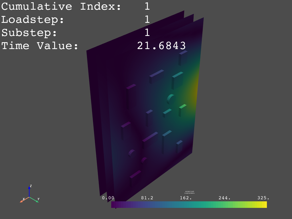
20.3.2.2. Using DPF-Post#
from ansys.dpf import post

solution_path = mapdl.result_file
solution = post.load_solution(solution_path)
print(solution)
displacement = solution.displacement(time_scoping=1)
total_deformation = displacement.norm
total_deformation.plot_contour(show_edges=True, background="w")
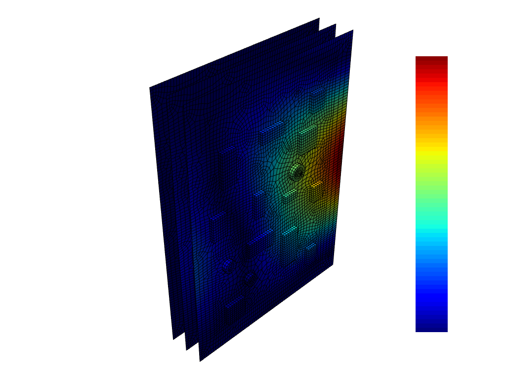
Modal analysis solution object.


Data Sources
------------------------------
DPF  DataSources:
  Result files:
     result key: rst and path: C:/Users/gayuso/AppData/Local/Temp/ansys_pasiuwhdkb\file.rst
  Secondary files:


DPF Model
------------------------------
Modal analysis
Unit system: NMM: mm, ton, N, s, mA, degC
Physics Type: Mecanic
Available results:
     -  displacement: Nodal Displacement
------------------------------
DPF  Meshed Region:
  44097 nodes
  26046 elements
  Unit: mm
  With solid (3D) elements, shell (2D) elements, shell (3D) elements, beam (1D) elements
------------------------------
DPF  Time/Freq Support:
  Number of sets: 10
Cumulative     Frequency (Hz) LoadStep       Substep
1              21.684283      1              1
2              21.690242      1              2
3              21.691317      1              3
4              33.829735      1              4
5              33.837985      1              5
6              33.839387      1              6
7              37.060643      1              7
8              37.070912      1              8
9              37.071871      1              9
10             43.837536      1              10

This may contain complex results.
20.3.2.3. Using DPF-Core#
from ansys.dpf import core

model = core.Model(solution_path)
results = model.results
print(results)
displacements = results.displacement()
total_def = core.operators.math.norm_fc(displacements)
total_def_container = total_def.outputs.fields_container()
mesh = model.metadata.meshed_region
mesh.plot(total_def_container.get_field_by_time_id(1), theme=mytheme)
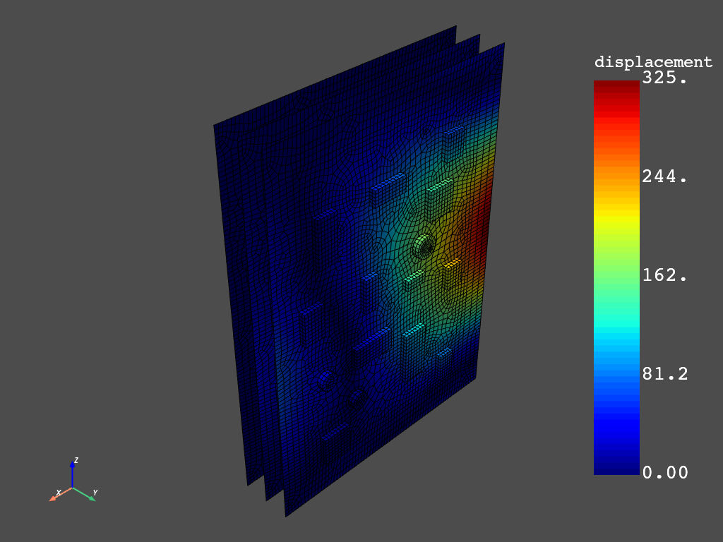
Modal analysis
Unit system: NMM: mm, ton, N, s, mA, degC
Physics Type: Mecanic
Available results:
     -  displacement: Nodal Displacement
20.4. PSD analysis#
20.4.1. Run PSD analysis#
The response spectrum analysis is defined, solved and post-processed.
# define PSD analysis with input spectrum
mapdl.slashsolu()
mapdl.antype("spectr")

# power spectral density
mapdl.spopt("psd")

# use input table 1 with acceleration spectrum in terms of acceleration due to gravity
mapdl.psdunit(1, "accg", 9.81 * 1000)

# define the frequency points in the input table 1
mapdl.psdfrq(1, "", 1, 40, 50, 70.71678, 100, 700, 900)

# define the PSD values in the input table 1
mapdl.psdval(1, 0.01, 0.01, 0.1, 1, 10, 10, 1)

# set the damping ratio as 5%
mapdl.dmprat(0.05)

# apply base excitation on the set of nodes N_BASE_EXCITE in the y-direction from table 1
mapdl.d("N_BASE_EXCITE", "uy", 1)

# calculate the participation factor for PSD with base excitation from input table 1
mapdl.pfact(1, "base")

# write the displacent solution relative to the base excitation to the results file from the PSD analysis
mapdl.psdres("disp", "rel")

# write the absolute velocity solution to the results file from the PSD analysis
mapdl.psdres("velo", "abs")

# write the absolute acceleration solution to the results file from the PSD analysis
mapdl.psdres("acel", "abs")

# combine only those modes whose significance level exceeds 0.0001
mapdl.psdcom()
output = mapdl.solve()
print(output)
*** NOTE *** CP = 16.328 TIME= 06:53:12
The automatic domain decomposition logic has selected the MESH domain
decomposition method with 2 processes per solution.
***** ANSYS SOLVE COMMAND *****
Time at start of random vibration closed-form solution CP= 16.328125.
FREQUENCIES USED FOR RANDOM VIBRATION SOLUTION
MODE FREQUENCY
1 21.6843
2 21.6902
3 21.6913
4 33.8297
5 33.8380
6 33.8394
7 37.0606
8 37.0709
9 37.0719
10 43.8375
PERFORM INTEGRATION FOR DISPLACEMENT-TYPE QUANTITIES
PERFORM INTEGRATION FOR VELOCITY-TYPE QUANTITIES
PERFORM INTEGRATION FOR ACCELERATION-TYPE QUANTITIES
Modal covariance matrix computed CP= 16.328125.
Quasi-static modal covariance matrix computed CP= 16.328125.
Covariant-modal covariance matrix computed CP= 16.328125.
Psd file file0.psd created. CP= 16.328125.
Time at start of random vibration mode combinations CP= 16.328125.
BASE EXCITATION PROBLEM
***** SUMMARY OF TERMS INCLUDED IN MODE COMBINATIONS *****
(MODAL COVARIANCE MATRIX TERMS ONLY)
*** DISPLACEMENT-TYPE QUANTITY ***
MAXIMUM TERM = 0.73456E-04
MODE MODE COVARIANCE COVARIANCE
I J TERM RATIO
1 1 0.73456E-04 1.0000
2 1 0.33327E-04 0.45370
2 2 0.15120E-04 0.20584
3 1 0.50316E-04 0.68498
3 2 0.22828E-04 0.31078
3 3 0.34466E-04 0.46920
4 1 0.64485E-05 0.87787E-01
4 2 0.29267E-05 0.39843E-01
4 3 0.44189E-05 0.60158E-01
4 4 0.26183E-05 0.35644E-01
5 1 0.30932E-05 0.42109E-01
5 2 0.14039E-05 0.19112E-01
5 3 0.21196E-05 0.28856E-01
5 4 0.12558E-05 0.17096E-01
5 5 0.60234E-06 0.82001E-02
6 1 0.46985E-05 0.63964E-01
6 2 0.21325E-05 0.29031E-01
6 3 0.32198E-05 0.43833E-01
6 4 0.19076E-05 0.25969E-01
6 5 0.91495E-06 0.12456E-01
6 6 0.13898E-05 0.18920E-01
7 1 0.10933E-04 0.14884
7 2 0.49619E-05 0.67549E-01
7 3 0.74918E-05 0.10199
7 4 0.37206E-05 0.50651E-01
7 5 0.17855E-05 0.24307E-01
7 6 0.27124E-05 0.36925E-01
7 7 0.71392E-05 0.97190E-01
8 1 0.68895E-05 0.93791E-01
8 2 0.31268E-05 0.42567E-01
8 3 0.47210E-05 0.64270E-01
8 4 0.23433E-05 0.31900E-01
8 5 0.11245E-05 0.15309E-01
8 6 0.17083E-05 0.23256E-01
8 7 0.44986E-05 0.61241E-01
8 8 0.28346E-05 0.38590E-01
9 1 0.99875E-05 0.13597
9 2 0.45329E-05 0.61708E-01
9 3 0.68440E-05 0.93171E-01
9 4 0.33968E-05 0.46243E-01
9 5 0.16301E-05 0.22192E-01
9 6 0.24763E-05 0.33712E-01
9 7 0.65214E-05 0.88780E-01
9 8 0.41093E-05 0.55942E-01
9 9 0.59571E-05 0.81098E-01
10 1 0.23871E-04 0.32496
10 2 0.10834E-04 0.14748
10 3 0.16357E-04 0.22268
10 4 0.70587E-05 0.96095E-01
10 5 0.33864E-05 0.46101E-01
10 6 0.51441E-05 0.70030E-01
10 7 0.12750E-04 0.17358
10 8 0.80366E-05 0.10941
10 9 0.11651E-04 0.15861
10 10 0.36571E-04 0.49786
*** VELOCITY-TYPE QUANTITY ***
MAXIMUM TERM = 15.547
MODE MODE COVARIANCE COVARIANCE
I J TERM RATIO
1 1 15.547 1.0000
2 1 7.0557 0.45383
2 2 3.2021 0.20596
3 1 10.653 0.68521
3 2 4.8347 0.31097
3 3 7.2996 0.46952
4 1 3.8958 0.25058
4 2 1.7681 0.11372
4 3 2.6695 0.17171
4 4 1.0786 0.69377E-01
5 1 1.8688 0.12020
5 2 0.84811 0.54551E-01
5 3 1.2805 0.82365E-01
5 4 0.51739 0.33279E-01
5 5 0.24818 0.15963E-01
6 1 2.8387 0.18259
6 2 1.2883 0.82864E-01
6 3 1.9451 0.12511
6 4 0.78592 0.50551E-01
6 5 0.37699 0.24249E-01
6 6 0.57266 0.36834E-01
7 1 6.5885 0.42378
7 2 2.9901 0.19233
7 3 4.5146 0.29039
7 4 1.7955 0.11549
7 5 0.86132 0.55401E-01
7 6 1.3084 0.84155E-01
7 7 3.0886 0.19866
8 1 4.1517 0.26704
8 2 1.8842 0.12119
8 3 2.8448 0.18298
8 4 1.1314 0.72770E-01
8 5 0.54272 0.34908E-01
8 6 0.82441 0.53027E-01
8 7 1.9463 0.12519
8 8 1.2264 0.78885E-01
9 1 6.0186 0.38712
9 2 2.7315 0.17569
9 3 4.1241 0.26527
9 4 1.6401 0.10549
9 5 0.78677 0.50606E-01
9 6 1.1951 0.76872E-01
9 7 2.8215 0.18148
9 8 1.7779 0.11436
9 9 2.5774 0.16578
10 1 13.822 0.88902
10 2 6.2727 0.40347
10 3 9.4709 0.60918
10 4 3.7285 0.23982
10 5 1.7885 0.11504
10 6 2.7168 0.17475
10 7 6.3657 0.40945
10 8 4.0114 0.25802
10 9 5.8153 0.37404
10 10 14.121 0.90826
*** ACCELERATION-TYPE QUANTITY ***
MAXIMUM TERM = 0.36471E+08
MODE MODE COVARIANCE COVARIANCE
I J TERM RATIO
1 1 0.36471E+08 1.0000
2 1 0.16552E+08 0.45383
2 2 0.75116E+07 0.20596
3 1 0.24990E+08 0.68521
3 2 0.11341E+08 0.31097
3 3 0.17124E+08 0.46952
4 1 0.93868E+07 0.25738
4 2 0.42600E+07 0.11680
4 3 0.64320E+07 0.17636
4 4 0.24200E+07 0.66353E-01
5 1 0.45026E+07 0.12346
5 2 0.20434E+07 0.56028E-01
5 3 0.30852E+07 0.84593E-01
5 4 0.11608E+07 0.31827E-01
5 5 0.55679E+06 0.15267E-01
6 1 0.68394E+07 0.18753
6 2 0.31039E+07 0.85106E-01
6 3 0.46865E+07 0.12850
6 4 0.17632E+07 0.48346E-01
6 5 0.84577E+06 0.23190E-01
6 6 0.12847E+07 0.35226E-01
7 1 0.15678E+08 0.42987
7 2 0.71150E+07 0.19509
7 3 0.10743E+08 0.29455
7 4 0.40413E+07 0.11081
7 5 0.19385E+07 0.53152E-01
7 6 0.29446E+07 0.80738E-01
7 7 0.67544E+07 0.18520
8 1 0.98787E+07 0.27086
8 2 0.44832E+07 0.12293
8 3 0.67690E+07 0.18560
8 4 0.25465E+07 0.69822E-01
8 5 0.12215E+07 0.33491E-01
8 6 0.18554E+07 0.50874E-01
8 7 0.42560E+07 0.11670
8 8 0.26818E+07 0.73531E-01
9 1 0.14321E+08 0.39266
9 2 0.64992E+07 0.17820
9 3 0.98129E+07 0.26906
9 4 0.36916E+07 0.10122
9 5 0.17707E+07 0.48552E-01
9 6 0.26898E+07 0.73750E-01
9 7 0.61698E+07 0.16917
9 8 0.38877E+07 0.10660
9 9 0.56359E+07 0.15453
10 1 0.31765E+08 0.87095
10 2 0.14416E+08 0.39526
10 3 0.21766E+08 0.59679
10 4 0.81902E+07 0.22457
10 5 0.39286E+07 0.10772
10 6 0.59676E+07 0.16362
10 7 0.13688E+08 0.37532
10 8 0.86252E+07 0.23649
10 9 0.12504E+08 0.34284
10 10 0.27823E+08 0.76287
***** SUMMARY OF OUTPUT QUANTITIES COMPUTED *****
AND WRITTEN ON RESULTS FILE
DISPLACEMENT-TYPE QUANTITIES COMPUTED
AND WRITTEN ON RESULTS FILE AS LOAD STEP 3
VALUES ARE RELATIVE TO BASE
THESE ARE STATISTICAL QUANTITIES WHICH
CANNOT BE COMBINED OR TRANSFORMED IN ANY
VECTORIAL SENSE
VELOCITY-TYPE QUANTITIES COMPUTED
AND WRITTEN ON RESULTS FILE AS LOAD STEP 4
VALUES ARE ABSOLUTE
THESE ARE STATISTICAL QUANTITIES WHICH
CANNOT BE COMBINED OR TRANSFORMED IN ANY
VECTORIAL SENSE
ACCELERATION-TYPE QUANTITIES COMPUTED
AND WRITTEN ON RESULTS FILE AS LOAD STEP 5
VALUES ARE ABSOLUTE
THESE ARE STATISTICAL QUANTITIES WHICH
CANNOT BE COMBINED OR TRANSFORMED IN ANY
VECTORIAL SENSE
20.4.2. Post-process PSD analysis#
The response spectrum analysis is post-processed. First, the standard MAPDL POST1 postprocessor is used. Then, the MAPDL time-history POST26 postprocessor is used to generate the response power spectral density.
Note
The graph generated through POST26 is exported as a picture in the working directory. Finally, the results from POST26 are saved to Python variables to be plotted in the Python environment with the use of Matplotlib library.
20.4.2.1. Post-process PSD analysis in POST1#
mapdl.post1()
mapdl.set(1, 1)
mapdl.plnsol("u", "sum")
mapdl.set("last")
mapdl.plnsol("u", "sum")
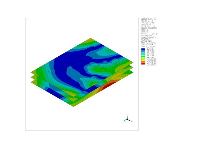
20.4.2.2. Post-process PSD analysis in POST26 (time-history post-processing)#
mapdl.post26()

# allow storage for 200 variables
mapdl.numvar(200)
mapdl.cmsel("s", "MY_MONITOR")
monitored_node = mapdl.queries.ndnext(0)
mapdl.store("psd")

# store the psd analysis u_y data for the node MYMONITOR as the reference no 2
mapdl.nsol(2, monitored_node, "u", "y")

# compute the response power spectral density for displacement associated with variable 2
mapdl.rpsd(3, 2)
mapdl.show("png")

# plot the variable 3
mapdl.plvar(3)

# print the variable 3
mapdl.prvar(3)

# x-axis is set for Log X scale
mapdl.gropt("logx", 1)

# y-axis is set for Log X scale
mapdl.gropt("logy", 1)

# plot the variable 3
mapdl.plvar(3)
mapdl.show("close")
20.4.2.3. Post-process PSD analysis using Matplotlib#
# store MAPDL results to python variables
mapdl.dim("frequencies", "array", 4000, 1)
mapdl.dim("response", "array", 4000, 1)
mapdl.vget("frequencies(1)", 1)
mapdl.vget("response(1)", 3)
frequencies = mapdl.parameters["frequencies"]
response = mapdl.parameters["response"]

# use Matplotlib to create graph
fig = plt.figure()
ax = fig.add_subplot(111)
plt.xscale("log")
plt.yscale("log")
ax.plot(frequencies, response)
ax.set_xlabel("Frequencies")
ax.set_ylabel("Response power spectral density")
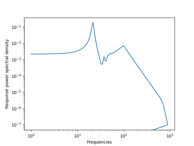
20.5. Exit MAPDL#
mapdl.exit()
20.6. Input files#
The following file was used in this problem:
pcb_mesh_file.cdb contains a FE model of a single
circuit board
pcb_mesh_file.cdb – Input file containing the model of a single circuit board.
For more information, see Obtaining the input files.