Brake squeal analysis#
This example analysis shows how to solve a brake-squeal problem. 1.6. Analysis and solution controls are highlighted: linear non-prestressed modal, partial nonlinear perturbed modal, and full nonlinear perturbed modal. The problem demonstrates sliding frictional contact and uses complex eigensolvers to predict unstable modes.
The following topics are available:
You can also perform this example analysis entirely in the Ansys Mechanical Application. For more information, see brake-squeal analysis in the Workbench technology showcase: example problems.
1.1. Introduction#
Eliminating brake noise is a classic challenge in the automotive industry. Brake discs develop large and sustained friction-induced oscillations, simple referred to as brake squeal.
Two common theories describe brake-squeal phenomena:
Stick-slip theory – The self-excited vibration of a brake system occurs when the static coefficient of friction is greater than the sliding coefficient of friction. Variable friction forces introduce energy into the system which is not properly dissipated during the squealing event, resulting in large vibrations.
Mode-coupling theory – When two similar characteristic modes couple with each other, instability is introduced to the braking system. This instability is caused primarily by improperly selected geometric parameters. Both theories attribute brake squeal to variable friction forces at the disc-pad interface.
Brake noise is generally categorized as follows:
Low-frequency noise – An example of a low-frequency noise is the “groaning” noise which occurs in the frequency range between 100 and 1000 Hz. Any noise having a frequency above 1000 Hz is considered a squeal.
Low-frequency squeal – A result of mode coupling occurring between the out-of-plane modes of the rotor and the bending modes of the brake pad.
High-frequency squeal – A result of mode coupling occurring between the in-plane modes of the rotor. Low- and high-frequency squealing can be determined via complex eigensolvers. The presence of unstable modes suggests that the geometry parameters and material properties of the braking system should be modified.
For more information, see brake-squeal (prestressed modal) analysis in the structural analysis guide.
1.2. Problem description#
The following model is a simple brake disc-pad assembly. The disc has a thickness of 10 mm and the brake pads have a thickness of 15 mm. The inner diameter of the disc is 250 mm and outer diameter is of 350 mm. A pre-stressed modal analysis is performed on this model using various methods to determine the unstable modes. A parametric study is then performed to examine the effect of the friction coefficient on the dynamic stability of the model.
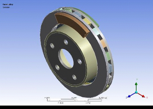
Fig. 6 Figure 1.1: Brake disc-pad assembly#
1.3. Modeling#
The following modeling topics are available:
1.3.1. Understanding the advantages of contact element technology#
Brake-squeal problems typically require manual calculations of the unsymmetric
terms arising from sources such as frictional sliding, and then inputting the
unsymmetric terms using special elements (such as
MATRIX27). It is a tedious process requiring a matched mesh
at the disc-pad interface along with assumptions related to the amount of area in
contact and sliding.
3-D contact elements (CONTA17x) offer a more efficient alternative by modeling
surface-to-surface contact at the pad-disc interface. With contact
surface-to-surface contact elements, a matched mesh is unnecessary at the
contact-target surface, and there is no need to calculate the unsymmetric
terms.
Contact surface-to-surface elements offer many controls for defining contact pairs, such as the type of contact surface, algorithm, contact stiffness, and gap/initial penetration effect.
1.3.2. Modeling contact pairs#
Frictional surface-to-surface contact pairs with a 0.3 coefficient of friction are used to define contact between the brake pads and disc to simulate frictional sliding contact occurring at the pad-disc interface. Bonded surface-to-surface contact pairs are used to define the contact for other components which will be always in contact throughout the braking operation.
The augmented Lagrange algorithm is used for the frictional contact pairs, as the pressure and frictional stresses are augmented during equilibrium iterations in such a way that the penetration is reduced gradually. The augmented Lagrange algorithm also requires fewer computational resources than the standard Lagrange multiplier algorithm, which normally requires additional iterations to ensure that the contact compatibility is satisfied exactly. The augmented Lagrange is well suited for modeling general frictional contact, such as the contact between the brake pad and disc defined in this example.
An internal multipoint constraint (MPC) contact algorithm is used for bonded contact because it ties contact and target surface together efficiently for solid-solid assembly. The MPC algorithm builds equations internally based on the contact kinematics and does not require the degrees of freedom of the contact surface nodes, reducing the wave front size of the equation solver. A contact detection point is made on the Gauss point for frictional contact pairs, and on the nodal point (normal-to-target surface) for MPC bonded contact pairs.
1.3.3. Generating internal sliding motion#
The Mapdl.cmrotate()
command defines constant rotational velocities on
the contact/target nodes to generate internal sliding motion. The specified
rotational velocity is used only to determine the sliding direction and has no
effect on the final solution. The element component used should include only the
contact or the target elements that are on the brake disc/rotor. In this example,
the target elements are defined on the disc surface and the contact elements are
defined on the pad surface. The target elements attached to the disc surface are
grouped to form a component named E_ROTOR which is then later specified on the
Mapdl.cmrotate()
command to generate a sliding frictional force.
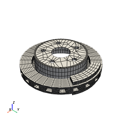
1.3.4. Meshing the brake disc-pad model#
The sweep method is used to generate a hexahedral dominant mesh of the brake
system assembly. Brake discs, pads and all other associated components are meshed
with 20-node structural solid SOLID186 elements with
uniform reduced-integration element technology. The edge sizing tool is used to
obtains a refined mesh at the pad-disc interface to improve the solution accuracy.
For problems with a large unsymmetric coefficient, a finer mesh should be used at
the pad-disc interface to accurately predict the unstable modes.
CONTA174 (3-D 8 node surface to surface contact)
elements are used to define the contact surface and
TARGE170 (3-D target segment) elements are used to
define the target surface. The brake disc-pad assembly is meshed with total of 60351
nodes and 11473 elements.
Start this example by launching MAPDL and loading the model.
# sphinx_gallery_thumbnail_path = '_static/tse1_setup.png'

import pyvista
pyvista.set_plot_theme('document')

from ansys.mapdl.core import launch_mapdl, Mapdl
from ansys.mapdl.core.examples.downloads import download_tech_demo_data
from ansys.mapdl.core.examples.examples import ansys_colormap

cdb_path = download_tech_demo_data("td-1", "disc_pad_model.cdb")

def start(mapdl, case):
    """Initialize MAPDL with a fresh disc pad model"""
    mapdl.finish()
    mapdl.verify(case)
    mapdl.prep7()
    mapdl.shpp("OFF", value2="NOWARN")  # disable element shape checking
    mapdl.cdread("COMB", cdb_path)  # Read disc_pad_model.cdb file
    mapdl.allsel()


mapdl = launch_mapdl(nproc=8)
mapdl.clear()

start(mapdl, 'linear_non_prestressed')
mapdl.title("linear_non_prestressed, Solving brake squeal problem using linear non pre-stressed modal solve")

mapdl.eplot(
    vtk=True, cpos="xy", show_edges=True, show_axes=False, line_width=2, background="w"
)
1.4. Material properties#
Linear elastic isotropic materials are assigned to all the components of the braking system.
Table 1.1: Material properties
Material properties |
|
|---|---|
Young’s Modulus (Nm-2) |
2.0 E+11 Pa |
Density |
7800 Kg/m3 |
Poisson’s Ratio |
0.3 |
1.5. Boundary conditions and loading#
The inner diameter of the cylinder hub and bolt holes is constrained in all directions. Small pressure loading is applied on both ends of the pad to establish contact with the brake disc and to include prestress effects. The displacement on the brake pad surfaces where the pressure loading is applied is constrained in all directions except axial (along the Z-axis).
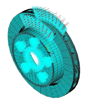
Fig. 7 Figure 1.2: Boundary conditions (displacement constraints and pressure loading)#
1.6. Analysis and solution controls#
The analysis settings and solution controls differ depending upon the method used to solve a brake-squeal problem. This section describes three possible methods:
1.6.1. Linear non-prestressed modal analysis#
A linear non-prestressed modal analysis is effective when the stress-stiffening effects are not critical. This method requires less run time than the other two methods, as Newton-Raphson iterations are not required. The contact-stiffness matrix is based on the initial contact status.
Following is the process for solving a brake-squeal problem using this method:
Perform a linear partial-element analysis with no prestress effects.
Generate the unsymmetric stiffness matrix (
Mapdl.nropt("UNSYM")).Generate sliding frictional force (
Mapdl.cmrotate()).Perform a complex modal analysis using the QRDAMP or UNSYM eigensolver.
When using the QRDAMP solver, you can reuse the symmetric eigensolution from the previous load steps (
Mapdl.qrdopt()), effective when performing a friction- sensitive/parametric analysis, as it saves time by not recalculating the real symmetric modes after the first solve operation.Expand the modes and postprocess the results from jobname.rST.
For this analysis, the UNSYM solver is selected to solve the problem. (Guidelines for selecting the eigensolver for brake-squeal problems appear in 1.8. Recommendations.)
The frequencies obtained from the modal solution have real and imaginary parts due the presence of an unsymmetric stiffness matrix. The imaginary frequency reflects the damped frequency, and the real frequency indicates whether the mode is stable or not. A real eigenfrequency with a positive value indicates an unstable mode.
The following input shows the solution steps involved in this method:
Modal solution
mapdl.run("/SOLU")
mapdl.nropt("UNSYM")  # To generate non symmetric
mapdl.cmsel("S", "C1_R")  # Select the target elements of the disc
mapdl.cmsel("A", "C2_R")
mapdl.cm("E_ROTOR", "ELEM")  # Form a component named E_ROTOR with the selected target elements
mapdl.allsel("ALL")
mapdl.cmrotate("E_ROTOR", "", "", 2)  # Rotate the selected element along global Z using CMROTATE command

# Perform modal solve, use UNSYM to extract 30 modes, and expand those
# modes.
mapdl.modal_analysis("UNSYM", 30, mxpand=True)
mapdl.finish()

mapdl.post1()
modes = []
modes.append(mapdl.set("list"))
mapdl.set(1, 21)

# Plot the mode shape for mode 21
mapdl.post_processing.plot_nodal_displacement(
    "NORM",
    cmap=ansys_colormap(),
    line_width=5,
    cpos="xy",
    scalar_bar_args={"title": "Displacement", "vertical": False},
)

Figure 1.3: Mode shape for unstable mode (Mode 21). Obtained from the 1.6.1. Linear non-prestressed modal analysis .
1.6.2. Partial nonlinear perturbed modal analysis#
Use a partial nonlinear perturbed modal analysis when stress-stiffening affects the final modal solution. The initial contact conditions are established, and a prestressed matrix is generated at the end of the first static solution.
Following is the process for solving a brake-squeal problem using this method:
Perform a nonlinear, large-deflection static analysis (
Mapdl.nlgeom("ON")).Use the unsymmetric Newton-Raphson method (
Mapdl.nropt("UNSYM")). Specify the restart control points needed for the linear perturbation analysis (Mapdl.rescontrol())Create components for use in the next step.
The static solution with external loading establishes the initial contact condition and generates a prestressed matrix.
Restart the previous static solution from the desired load step and substep, and perform the first phase of the perturbation analysis while preserving the .ldhi, .rnnn and .rst files (
Mapdl.antype("STATIC", "RESTART", "", "", "PERTURB")).Initiate a modal linear perturbation analysis (
Mapdl.perturb("MODAL")).Generate forced frictional sliding contact (
Mapdl.cmrotate()), specifying the component names created in the previous step.The contact stiffness matrix is based only on the contact status at the restart point.
Regenerate the element stiffness matrix at the end of the first phase of the linear perturbation solution (
Mapdl.solve("ELFORM")).Obtain the linear perturbation modal solution using the QRDAMP or UNSYM eigensolver (
Mapdl.modopt()).When using the QRDAMP solver, you can reuse the symmetric eigensolution from the previous load steps (
Mapdl.qrdopt()), effective when performing a friction-sensitive/parametric analysis, as it saves time by not recalculating the real symmetric modes after the first solve operation.Expand the modes and postprocess the results (from the jobname.rstp file).
The following inputs show the solution steps involved with this method:
Static solution
start(mapdl, "partial_prestressed")
mapdl.title("partial_prestressed, Solving brake squeal problem using partial pre-stressed modal solve")

mapdl.run("/SOLU")
mapdl.antype("STATIC")  # Perform static solve
mapdl.outres("ALL", "ALL")  # Write all element and nodal solution results for each sub steps
mapdl.nropt("UNSYM")  # Specify unsymmetric Newton-Raphson option to solve the problem
mapdl.rescontrol("DEFINE", "ALL", 1)  # Control restart files
mapdl.nlgeom("ON")  # Activate large deflection
mapdl.autots("ON")  # Auto time stepping turned on
mapdl.time(1.0)  # End time = 1.0 sec
mapdl.esel("S", "TYPE", "", 124)  # Select element type 124
mapdl.nsle("S", "ALL")  # Select nodes attached to the element
mapdl.sf("ALL", "PRES", "%_LOADVARI4059%")  # Apply surface pressure on the selected nodes
mapdl.esel("S", "TYPE", "", 125)  # Select element type 125
mapdl.nsle("S", "ALL")  # Select nodes attached to the element
mapdl.sf("ALL", "PRES", "%_LOADVARI4061%")  # Apply surface pressure on the selected nodes
mapdl.nsel("ALL")
mapdl.allsel("ALL")
mapdl.cmsel("S", "C1_R")  # Select target elements of the disc
mapdl.cmsel("A", "C2_R")
mapdl.cm("E_ROTOR", "ELEM")  # Form a component named E_ROTOR
mapdl.allsel("ALL")
mapdl.solve()  # Solve with prestress
mapdl.finish()
Post processing to show partial results.
# select contact elements attached to the brake pad
mapdl.post1()
mapdl.set("last")
mapdl.esel("s", "type", "", 30, 32, 2)
mapdl.post_processing.plot_element_values(
    "CONT", "STAT", scalar_bar_args={"title": "Contact status"}
)

mapdl.post_processing.plot_element_values(
    "CONT", "SLIDE", scalar_bar_args={"title": "Contact sliding distance"}
)

mapdl.allsel("all")
mapdl.finish()
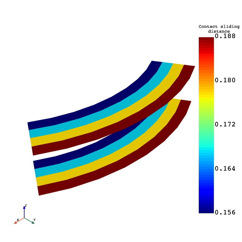
Fig. 8 Figure 1.4: Contact sliding distance#
Perturbed modal solution
# Restart from last load step and sub step of previous
mapdl.run("/SOLU")
mapdl.antype("static", "restart", "", "", "perturb")

# static solution to perform perturbation analysis
mapdl.perturb("modal", "", "", "")  # Perform perturbation modal solve
mapdl.cmrotate("E_ROTOR", rotatz=2)
mapdl.solve("elform")  # Regenerate the element matrices
mapdl.outres("all", "all")
mapdl.modopt("unsym", 30)  # Use UNSYM eigen solver and extract 30 modes
mapdl.mxpand(30, "", "", "")  # Expand 30 modes
mapdl.solve()
mapdl.finish()
Post processing to show results.
mapdl.post1()
mapdl.file("", "rstp")
print(mapdl.post_processing)

mapdl.set(1, 21)
mapdl.post_processing.plot_nodal_displacement(
    scalar_bar_args={"title": "Total displacement\n Substep 21"}
)

mapdl.set(1, 22)
mapdl.post_processing.plot_nodal_displacement(
    scalar_bar_args={"title": "Total displacement\n Substep 22"}
)
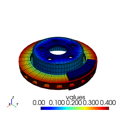
Figure 1.5: Mode shape for unstable mode (Mode 21). Obtained from the 1.6.1. Linear non-prestressed modal analysis .
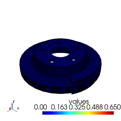
Figure 1.6: Mode shape for unstable mode (Mode 21). Obtained from the 1.6.1. Linear non-prestressed modal analysis .
1.6.3. Full nonlinear perturbed modal analysis#
A full nonlinear perturbed modal analysis is the most accurate method for modeling the brake-squeal problem. This method uses Newton-Raphson iterations for both of the static solutions.
Following is the process for solving a brake-squeal problem using this method:
Perform a nonlinear, large-deflection static analysis (
Mapdl.nlgeom("ON")). Use the unsymmetric Newton-Raphson method (Mapdl.nropt("UNSYM")). Specify the restart control points needed for the linear perturbation analysis (Mapdl.rescontrol()).Perform a full second static analysis. Generate sliding contact (
Mapdl.cmrotate()) to form an unsymmetric stiffness matrix.After obtaining the second static solution, postprocess the contact results. Determine the status (that is, whether the elements are sliding, and the sliding distance, if any).
Restart the previous static solution from the desired load step and substep, and perform the first phase of the perturbation analysis while preserving the .ldhi, .rnnn and .rst files (
Mapdl.antype("STATIC", "RESTART",,, "PERTURB")).Initiate a modal linear perturbation analysis (
Mapdl.perturb("MODAL")).Regenerate the element stiffness matrix at the end of the first phase of the linear perturbation solution (
Mapdl.solve("ELFORM")).Obtain the linear perturbation modal solution using the QRDAMP or UNSYM eigensolver (
Mapdl.modopt()).Expand the modes and postprocess the results (from the jobname.rstp file). The following inputs show the solution steps involved with this method:
First static solution
start(mapdl, 'full_non_linear')

mapdl.run("/SOLU")
mapdl.antype("STATIC")  # Perform static solve
mapdl.outres("ALL", "ALL")  # Write all element and nodal solution results for each substep
mapdl.nropt("UNSYM")  # Specify unsymmetric Newton-Raphson option to solve the problem
mapdl.rescontrol("DEFINE", "ALL", 1)  # Control restart files
mapdl.nlgeom("ON")  # Activate large deflection
mapdl.autots("ON")  # Auto time stepping turned on
mapdl.time(1.0)  # End time = 1.0 sec
mapdl.esel("S", "TYPE", "", 124)  # Select element type 124
mapdl.nsle("S", "ALL")  # Select nodes attached to the element
mapdl.sf("ALL", "PRES", "%_LOADVARI4059%")  # Apply surface pressure on the selected nodes
mapdl.esel("S", "TYPE", "", 125)  # Select element type 125
mapdl.nsle("S", "ALL")  # Select nodes attached to the element
mapdl.sf("ALL", "PRES", "%_LOADVARI4061%")  # Apply surface pressure on the selected nodes
mapdl.nsel("ALL")
mapdl.allsel("ALL")
mapdl.cmsel("S", "C1_R")  # Select the target elements of the disc
mapdl.cmsel("A", "C2_R")
mapdl.cm("E_ROTOR", "ELEM")  # Form a component named E_ROTOR with the selected target ELEMENTS
mapdl.allsel("ALL")
mapdl.solve()  # Solve with prestress loading
Second static solution
mapdl.cmrotate("E_ROTOR", rotatz=2)
mapdl.time(2.0)  # End time = 2.0sec
mapdl.solve()  # Perform full solve
mapdl.finish()
Plotting partial results
mapdl.post1()
mapdl.set("last")

# select contact elements attached to the brake pad
mapdl.esel("s", "type", "", 30, 32, 2)

mapdl.post_processing.plot_element_values(
    "CONT", "STAT", scalar_bar_args={"title": "Contact status"}
)

mapdl.post_processing.plot_element_values(
    "CONT", "SLIDE", scalar_bar_args={"title": "Contact sliding distance"}
)

mapdl.allsel("all")
mapdl.finish()
Perturbed modal solution
mapdl.run("/SOLU")
mapdl.antype("STATIC", "RESTART", action="PERTURB")  # Restart from last load step and sub step
mapdl.perturb("MODAL")  # Perform linear perturbation modal solve
mapdl.solve("ELFORM")  # Regenerate the element stiffness matrix
mapdl.outres("ALL", "ALL")
mapdl.modopt("UNSYM", 30)  # Use UNSYM eigensolver and extract 30 modes
mapdl.mxpand(30)  # Expand 30 modes
mapdl.solve()  # Solve linear perturbation modal solve
Plotting results
mapdl.post1()
mapdl.file("", "RSTP")
print(mapdl.post_processing)


mapdl.set(1, 21)
mapdl.post_processing.plot_nodal_displacement(
    scalar_bar_args={"title": "Total displacement\n Substep 21"}
)

mapdl.set(1, 22)
mapdl.post_processing.plot_nodal_displacement(
    scalar_bar_args={"title": "Total displacement\n Substep 22"}
)

mapdl.finish()
mapdl.exit()
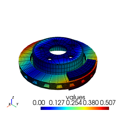
Figure 1.7: Mode shape for unstable mode (Mode 21).
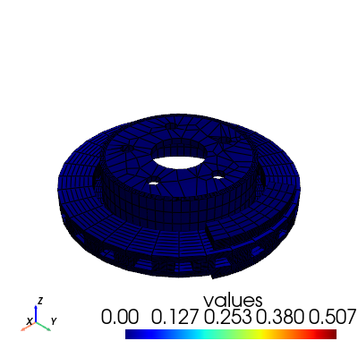
Figure 1.8: Mode shape for unstable mode (Mode 21).
1.7. Results and discussion#
The unstable mode predictions for the brake disc-pad assembly using all three methods were very close due to the relatively small prestress load. The 1.6.1. linear non-prestressed modal analysis predicted unstable modes at 6474 Hz, while the other two solution methods predicted unstable modes at 6470 Hz.
The mode shape plots for the unstable modes suggest that the bending mode of the pads and disc have similar characteristics. These bending modes couple due to friction, and produce a squealing noise.
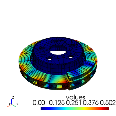
Figure 1.9: Mode shape for unstable mode (Mode 21). Obtained from the 1.6.1. Linear non-prestressed modal analysis .

Figure 1.10: Mode shape for unstable mode (Mode 22). Obtained from the 1.6.1. Linear non-prestressed modal analysis .
Table 1.2: Solution output
Linear non-prestressed modal |
Partial nonlinear perturbed modal |
Full nonlinear perturbed modal |
||||
|---|---|---|---|---|---|---|
Mode |
Imaginary |
Real |
Imaginary |
Real |
Imaginary |
Real |
1.00 |
775.91 |
0.00 |
775.73 |
0.00 |
775.73 |
0.00 |
2.00 |
863.54 |
0.00 |
863.45 |
0.00 |
863.45 |
0.00 |
3.00 |
1097.18 |
0.00 |
1097.03 |
0.00 |
1097.03 |
0.00 |
4.00 |
1311.54 |
0.00 |
1311.06 |
0.00 |
1311.06 |
0.00 |
5.00 |
1328.73 |
0.00 |
1328.07 |
0.00 |
1328.07 |
0.00 |
6.00 |
1600.95 |
0.00 |
1600.66 |
0.00 |
1600.66 |
0.00 |
7.00 |
1616.15 |
0.00 |
1615.87 |
0.00 |
1615.87 |
0.00 |
8.00 |
1910.50 |
0.00 |
1910.50 |
0.00 |
1910.50 |
0.00 |
9.00 |
2070.73 |
0.00 |
2070.44 |
0.00 |
2070.44 |
0.00 |
10.00 |
2081.26 |
0.00 |
2080.98 |
0.00 |
2080.98 |
0.00 |
11.00 |
2676.71 |
0.00 |
2675.23 |
0.00 |
2675.23 |
0.00 |
12.00 |
2724.05 |
0.00 |
2722.61 |
0.00 |
2722.61 |
0.00 |
13.00 |
3373.96 |
0.00 |
3373.32 |
0.00 |
3373.32 |
0.00 |
14.00 |
4141.64 |
0.00 |
4141.45 |
0.00 |
4141.45 |
0.00 |
15.00 |
4145.16 |
0.00 |
4145.04 |
0.00 |
4145.04 |
0.00 |
16.00 |
4433.91 |
0.00 |
4431.08 |
0.00 |
4431.08 |
0.00 |
17.00 |
4486.50 |
0.00 |
4484.00 |
0.00 |
4484.00 |
0.00 |
18.00 |
4668.51 |
0.00 |
4667.62 |
0.00 |
4667.62 |
0.00 |
19.00 |
4767.54 |
0.00 |
4766.95 |
0.00 |
4766.95 |
0.00 |
20.00 |
5241.61 |
0.00 |
5241.38 |
0.00 |
5241.38 |
0.00 |
21.00 |
6474.25 |
21.61 |
6470.24 |
21.90 |
6470.24 |
21.90 |
22.00 |
6474.25 |
-21.61 |
6470.24 |
-21.90 |
6470.24 |
-21.90 |
23.00 |
6763.36 |
0.00 |
6763.19 |
0.00 |
6763.19 |
0.00 |
24.00 |
6765.62 |
0.00 |
6765.51 |
0.00 |
6765.51 |
0.00 |
25.00 |
6920.64 |
0.00 |
6919.64 |
0.00 |
6919.64 |
0.00 |
26.00 |
6929.25 |
0.00 |
6929.19 |
0.00 |
6929.19 |
0.00 |
27.00 |
7069.69 |
0.00 |
7066.72 |
0.00 |
7066.72 |
0.00 |
28.00 |
7243.80 |
0.00 |
7242.71 |
0.00 |
7242.71 |
0.00 |
29.00 |
8498.41 |
0.00 |
8493.08 |
0.00 |
8493.08 |
0.00 |
30.00 |
8623.76 |
0.00 |
8616.68 |
0.00 |
8616.68 |
0.00 |
1.7.1. Determining the modal behavior of individual components#
It is important to determine the modal behavior of individual components (disc and pads) when predicting brake-squeal noise. A modal analysis performed on the free pad and free disc model gives insight into potential coupling modes. The natural frequency and mode shapes of brake pads and disc can also be used to define the type of squeal noise that may occur in a braking system. Bending modes of pads and disc are more significant than twisting modes because they eventually couple to produce squeal noise.
An examination of the results obtained from the modal analysis of a free disc and pad shows that the second bending mode of the pad and ninth bending mode of the disc can couple to create dynamic instability in the system. These pad and disc bending modes can couple to produce an intermediate lock, resulting in a squeal noise at a frequency close to 6470 Hz.
1.7.2. Parametric study with increasing friction coefficient#
A parametric study was performed on the brake disc model using a linear
non-prestressed modal solution with an increasing coefficient of friction. QRDAMP
eigensolver is used to perform the parametric studies by reusing the symmetric real
modes (Mapdl.qrdopt("ON")) obtained in the first load
step.
The following plot suggests that modes with similar characteristics approach each other and couple as the coefficient of friction increases:
Figure 1.11: Effect of friction coefficient on unstable modes
1.8. Recommendations#
The following table provides guidelines for selecting the optimal analysis method to use for a brake-squeal problem:
Table 1.3: Analysis comparison
Analysis method |
Benefits |
Costs |
|---|---|---|
Linear non-prestressed modal |
|
|
Partial nonlinear perturbed modal |
|
|
Full nonlinear perturbed modal |
|
|
The following table provides guidelines for selecting the optimal eigensolver
(Mapdl.modopt()) for obtaining the brake-squeal solution:
Table 1.4: Solver comparison
Eigensolver |
Benefits |
Costs |
|---|---|---|
QRDAMP |
|
|
UNSYM |
|
|
For further information, see Brake-Squeal (prestressed modal) Analysis in the structural analysis guide.
1.9. References#
The following works were consulted when creating this example problem:
Triches, M. Jr., Gerges, S. N. Y., & Jordon, R. (2004). Reduction of squeal noise from disc brake systems using constrained layer damping. Journal of the Brazilian Society of Mechanical Sciences and Engineering. 26, 340-343.
Allgaier, R., Gaul, L., Keiper, W., & Willner, K. (1999). Mode lock-in and friction modeling. Computational Methods in Contact Mechanics. 4, 35-47.
Schroth, R., Hoffmann, N., Swift, R. (2004, January). Mechanism of brake squeal from theory to experimentally measured mode coupling. In Proceedings of the twenty second International Modal Analysis Conference (IMAC XXII).
1.10. Input files#
The following input files were used for this problem:
linear_non_prestressed.html – Linear non-prestressed modal solve input file.
Download source code: linear_non_prestressed.py.partial_prestressed.html – Partial prestressed modal solve input file.
Download source code: partial_prestressed.py.full_non_linear.html – Full nonlinear prestressed modal solve input file.
Download source code: full_non_linear.py.linear_non_prestressed_par.html – Parametric studies with increasing coefficient of friction.
Download source code: linear_non_prestressed_par.py.disc_pad_model.cdb – Common database file used for the linear non-prestressed modal analysis, the partial prestressed modal analysis, and the full nonlinear prestressed modal analysis (called by the linear_non_prestressed.dat, partial_prestressed.dat, full_non_linear.html and linear_non_prestressed_par.html files, respectively).
Download file: disc_pad_model.cdb.
For more information, see Obtaining the input files.