Cardiovascular stent simulation#
This example problem shows how to simulate stent-artery interaction during and after stent placement in an occluded artery. The analysis exposes advanced modeling techniques using PyMAPDL such as: * Contact * Element birth and death * Mixed u-P formulation * Nonlinear stabilization
The following topics are available:
This example is inspired from the model and analysis defined in Chapter 25 of the Mechanical APDL technology showcase manual.
25.1. Introduction#
25.1.1. Problem description#
A bare metal stent is an effective device for opening atherosclerotic arteries and other blockages:
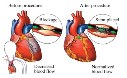
Fig. 19 Figure 25.1: Effect of stent placement in increasing blood flow Courtesy of Lakeview Center#
The success of stenting depends largely on how the stent and the artery interact mechanically. In both the stent-design process and in pre-clinical patient-specific evaluations, computer simulation using finite element analysis (FEA) has become an accepted tool for studying stent-artery interaction.
A viable stent-artery finite element model must properly reflect the nonlinear nature of the phenomenon, such as the biological tissue properties, large arterial wall deformation, and the sliding contact between the stent and the artery wall.
25.1.2. Starting MAPDL as a service#
# Starting MAPDL as a service and importing an external model
from ansys.mapdl.core import launch_mapdl

# Start MAPDL as a service
mapdl = launch_mapdl()
print(mapdl)
25.2. Setting up the model#
First, we define the material properties.
# define 316L stainless steel
mapdl.prep7()
mapdl.mptemp()
mapdl.mptemp(sloc="1", t1="0")
mapdl.mpdata(lab="EX", mat="1", c1="200e3")
mapdl.mpdata(lab="PRXY", mat="1", c1="0.3")
mapdl.mptemp()
mapdl.mptemp(sloc="1", t1="0")
mapdl.mpdata(lab="DENS", mat="1", c1="8000e-9")
Then, we can define the elements.
# for straight line segments
mapdl.et(itype="1", ename="beam189")
mapdl.sectype(secid="1", type_="beam", subtype="csolid")
mapdl.secdata(val1=0.05)

# for arcs
mapdl.et(itype="2", ename="beam189")
mapdl.sectype(secid="2", type_="beam", subtype="csolid")
mapdl.secdata(val1=0.05)
We define the 5-parameter Mooney-Rivlin hyperelastic artery material model.
c10 = 18.90e-3
c01 = 2.75e-3
c20 = 590.43e-3
c11 = 857.2e-3
nu1 = 0.49
dd = 2 * (1 - 2 * nu1) / (c10 + c01)

mapdl.tb(lab="hyper", mat="2", npts="5", tbopt="mooney")
mapdl.tbdata(stloc="1", c1="c10", c2="c01", c3="c20", c4="c11", c6="dd")
We define the linear elastic material model for stiff calcified plaque.
mapdl.mp(lab="EX", mat="3", c0=".00219e3")
mapdl.mp(lab="NUXY", mat="3", c0="0.49")
We define the Solid185 element type to mesh both the artery and plaque.
# for artery
mapdl.et(itype="9", ename="SOLID185")
mapdl.keyopt(
    itype="9", knum="6", value="1")  # Use mixed u-P formulation to avoid locking
mapdl.keyopt(itype="9", knum="2", value="3")  # Use simplified enhanced strain method

# for plaque
mapdl.et(itype="16", ename="SOLID185")
mapdl.keyopt(itype="16", knum="2", value="0")  # Use B-bar
We define the settings to model the stent, the artery and the plaque.
We use force-distributed boundary constraints on 2 sides of artery wall to allow for radial expansion of tissue without rigid body motion.
Settings for MPC surface-based, force-distributed contact on proximal plane parallel to x-y plane
mapdl.mat("2")
mapdl.r(nset="3")
mapdl.real(nset="3")
mapdl.et(itype="3", ename="170")
mapdl.et(itype="4", ename="174")
mapdl.keyopt(itype="4", knum="12", value="5")
mapdl.keyopt(itype="4", knum="4", value="1")
mapdl.keyopt(itype="4", knum="2", value="2")
mapdl.keyopt(itype="3", knum="2", value="1")
mapdl.keyopt(itype="3", knum="4", value="111111")
mapdl.type(itype="3")

mapdl.mat("2")
mapdl.r(nset="4")
mapdl.real(nset="4")
mapdl.et(itype="5", ename="170")
mapdl.et(itype="6", ename="174")
mapdl.keyopt(itype="6", knum="12", value="5")
mapdl.keyopt(itype="6", knum="4", value="1")
mapdl.keyopt(itype="6", knum="2", value="2")
mapdl.keyopt(itype="5", knum="2", value="1")
mapdl.keyopt(itype="5", knum="4", value="111111")
mapdl.type(itype="5")
Settings for standard contact between stent and inner plaque wall contact surface
mapdl.mp(lab="MU", mat="1", c0="0")
mapdl.mat("1")
mapdl.mp(lab="EMIS", mat="1", c0="7.88860905221e-31")
mapdl.r(nset="6")
mapdl.real(nset="6")
mapdl.et(itype="10", ename="170")
mapdl.et(itype="11", ename="177")
mapdl.r(nset="6", r3="1.0", r4="1.0", r5="0")
mapdl.rmore(r9="1.0E20", r10="0.0", r11="1.0")
mapdl.rmore(r7="0.0", r8="0", r9="1.0", r10="0.05", r11="1.0", r12="0.5")
mapdl.rmore(r7="0", r8="1.0", r9="1.0", r10="0.0")
mapdl.keyopt(itype="11", knum="5", value="0")
mapdl.keyopt(itype="11", knum="7", value="1")
mapdl.keyopt(itype="11", knum="8", value="0")
mapdl.keyopt(itype="11", knum="9", value="0")
mapdl.keyopt(itype="11", knum="10", value="2")
mapdl.keyopt(itype="11", knum="11", value="0")
mapdl.keyopt(itype="11", knum="12", value="0")
mapdl.keyopt(itype="11", knum="2", value="3")
mapdl.keyopt(itype="10", knum="5", value="0")
Settings for MPC based, force-distributed constraint on proximal stent nodes
mapdl.mat("1")
mapdl.r(nset="7")
mapdl.real(nset="7")
mapdl.et(itype="12", ename="170")
mapdl.et(itype="13", ename="175")
mapdl.keyopt(itype="13", knum="12", value="5")
mapdl.keyopt(itype="13", knum="4", value="1")
mapdl.keyopt(itype="13", knum="2", value="2")
mapdl.keyopt(itype="12", knum="2", value="1")
mapdl.keyopt(itype="12", knum="4", value="111111")
mapdl.type(itype="12")
Settings for MPC based, force-distributed constraint on distal stent nodes.
mapdl.mat("1")
mapdl.r(nset="8")
mapdl.real(nset="8")
mapdl.et(itype="14", ename="170")
mapdl.et(itype="15", ename="175")
mapdl.keyopt(itype="15", knum="12", value="5")
mapdl.keyopt(itype="15", knum="4", value="1")
mapdl.keyopt(itype="15", knum="2", value="2")
mapdl.keyopt(itype="14", knum="2", value="1")
mapdl.keyopt(itype="14", knum="4", value="111111")
mapdl.type(itype="14")
Once all the setups are ready, we read the geometry file.
mapdl.cdread(option="db", fname="stent", ext="cdb")
mapdl.allsel(labt="all")
mapdl.finish()
25.3. Analysis#
25.3.1. Static analysis#
We, then, apply the static analysis.
# Enter solution processor and define analysis settings
mapdl.run("/solu")
mapdl.antype(antype="0")
mapdl.nlgeom(key="on")
25.3.2. Loads#
We apply the load step 1: Balloon angioplasty of the artery to expand it past the radius of the stent - IGNORE STENT
mapdl.nsubst(nsbstp="20", nsbmx="20")
mapdl.nropt(option1="full")
mapdl.cncheck(option="auto")
mapdl.esel(type_="s", item="type", vmin="11")
mapdl.cm(cname="contact2", entity="elem")
mapdl.ekill(elem="contact2")  # Kill contact elements in stent-plaque contact
                              #pair so that the stent is ignored in the first loadstep
mapdl.nsel(type_="s", item="loc", comp="x", vmin="0", vmax="0.01e-3")
mapdl.nsel(type_="r", item="loc", comp="y", vmin="0", vmax="0.01e-3")
mapdl.d(node="all", lab="all")
mapdl.allsel()

mapdl.sf(nlist="load", lab="pres", value="10e-2")  # Apply 0.1 Pa/mm^2 pressure to inner plaque wall
mapdl.allsel()
mapdl.nldiag(label="cont", key="iter")
mapdl.solve()
mapdl.save()
We then apply the load step 2: Reactivate contact between stent and plaque.
mapdl.ealive(elem="contact2")
mapdl.allsel()

mapdl.nsubst(nsbstp="2", nsbmx="2")
mapdl.save()
mapdl.solve()
We apply the load step 3.
mapdl.nsubst(nsbstp="1", nsbmx="1", nsbmn="1")
mapdl.solve()
We apply the load step 4: Apply blood pressure (13.3 kPa) load to inner wall of plaque and allow the stent to act as a scaffold.
mapdl.nsubst(nsbstp="300", nsbmx="3000", nsbmn="30")
mapdl.sf(nlist="load", lab="pres", value="13.3e-3")
mapdl.allsel()
Finally, we apply stabilization with energy option.
mapdl.stabilize(key="const", method="energy", value="0.1")
25.4. Solution of the model#
mapdl.solve()
mapdl.save()
mapdl.finish()
25.5. Results#
This section illustrates the use of PyDPF-Core to post-process the results.
from ansys.dpf import core as dpf
from ansys.dpf.core import operators as ops
import pyvista
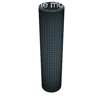
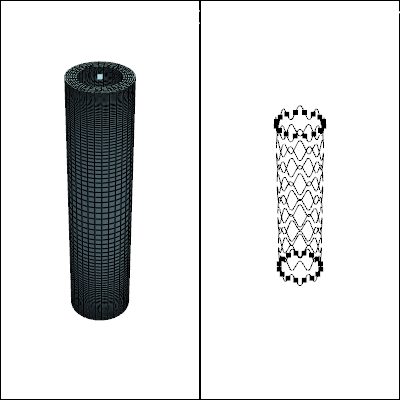
25.5.1. Mesh of the model#
# Loading the result file
model = dpf.Model(mapdl.result_file)
ds = dpf.DataSources(mapdl.result_file)

mesh = model.metadata.meshed_region
mesh.plot()
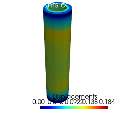
25.5.2. Computed displacements of the model#
# Collecting the computed displacement
u = model.results.displacement(time_scoping=[4]).eval()

u[0].plot(deform_by = u[0])
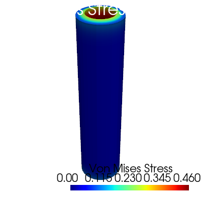
25.5.3. Von Mises stress#
# Collecting the computed stress
s_op = model.results.stress(time_scoping=[3])
s_op.inputs.requested_location.connect(dpf.locations.nodal)
s = s_op.eval()

# Calculating Von Mises stress
s_VM = dpf.operators.invariant.von_mises_eqv_fc(fields_container=s)
s_VM_plot = s_VM.eval()

s_VM_plot[0].plot(deform_by = u[0])
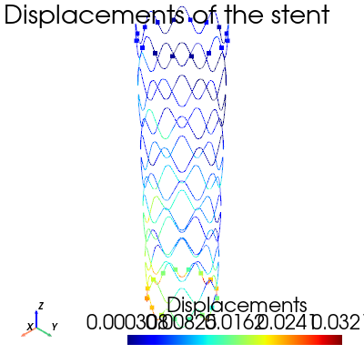
25.5.4. Computed displacements of the stent#
# Creating the mesh associated to the stent
esco = mesh.named_selection("STENT")
print(esco)

# Transposing elemental location to nodal one
op = dpf.operators.scoping.transpose()
op.inputs.mesh_scoping.connect(esco)
op.inputs.meshed_region.connect(mesh)
op.inputs.inclusive.connect(1)
nsco = op.eval()
print(nsco)
# Collecting the computed displacements of the stent
u_stent = model.results.displacement(mesh_scoping=nsco, time_scoping=[4])
u_stent = u_stent.outputs.fields_container()

# Linking the stent mesh to the global one
op = dpf.operators.mesh.from_scoping() # operator instantiation
op.inputs.scoping.connect(nsco)
op.inputs.inclusive.connect(1)
op.inputs.mesh.connect(mesh)
mesh_sco = op.eval()
u_stent[0].meshed_region = mesh_sco

# Plotting the meshes
mesh.plot(color="w", show_edges=True, text='Mesh of the model', )
mesh_sco.plot(color="black", show_edges=True, text='Mesh of the stent')
u_stent[0].plot(deformed_by=u_stent[0])
25.6. Exit MAPDL#
mapdl.exit()
25.7. Input files#
The following files were used in this problem:
stent.dat – Input file for the cardiovascular stent problem.
stent.cdb – The common database file containing the model information for this problem (called by stent.dat).
For more information, see Obtaining the input files.