Friction Stir Welding (FSW) simulation#
This example problem shows how to simulate the friction stir welding (FSW) process. Several characteristics of FSW are presented, including tool-workpiece surface interaction, heat generation due to friction, and plastic deformation. A nonlinear direct coupled-field analysis is performed, as thermal and mechanical behaviors are mutually dependent and coupled together during the FSW process.
Because it is often difficult to find a full set of engineering data to simulate the FSW process, the problem emphasizes the simulation rather than the numerical results. A simplified version of the model created by Zhu and Chao illustrates the FSW simulation method.
The following features and capabilities are highlighted:
Direct structural-thermal analysis using coupled-field solid elements
Plastic heat generation in coupled-field elements
Frictional heat generation using contact elements
Surface-projection-based contact method
Contact elements with bonding capability
The following topics are available:
You can also perform this example analysis entirely in the Ansys Mechanical Application. For more information, see Friction Stir Welding (FSW) Simulation in the Workbench Technology Showcase: example problems.
28.1. Introduction#
Friction Stir Welding (FSW) is a solid-state welding technique that involves the joining of metals without filler materials. A cylindrical rotating tool plunges into a rigidly clamped workpiece and moves along the joint to be welded. As the tool translates along the joint, heat is generated by friction between the tool shoulder and the workpiece. Additional heat is generated by plastic deformation of the workpiece material. The generated heat results in thermal softening of the workpiece material. The translation of the tool causes the softened workpiece material to flow from the front to the back of the tool where it consolidates. As cooling occurs, a solid continuous joint between the two plates is formed. No melting occurs during the process, and the resulting temperature remains below the solidus temperature of the metals being joined. FSW offers many advantages over conventional welding techniques, and has been successfully applied in the aerospace, automobile, and shipbuilding industries.
Thermal and mechanical behaviors are mutually dependent during the FSW process. Because the temperature field affects stress distribution, this example uses a fully thermomechanically coupled model. The model consists of a coupled-field solid element with structural and thermal degrees of freedom. The model has two rectangular steel plates and a cylindrical tool. All necessary mechanical and thermal 28.5. Boundary conditions and loading are applied on the model. The simulation occurs over three load steps, representing the 28.5.3. Loading of the process.
The temperature rises at the contact interface due to frictional contact between the tool and workpiece. FSW generally occurs when the temperature at the weld line region reaches 70 to 90 percent of the melting temperature of the workpiece material. The temperature obtained around the weld line region in this example falls within the range reported by Zhu and Chao [Zhu2004] and Prasanna and Rao [Prasanna2010], while the maximum resulting temperature is well below the melting temperature of the workpiece.
The calculated frictional heat generation and plastic heat generation show that the friction between the tool shoulder and workpiece is responsible for generating most of the heat. A bonding temperature is specified at the contact interface of the plates to model the welding behind the tool. When the temperature at the contact surface exceeds this bonding temperature, the contact is changed to bonded.
28.2. Problem description#
The Zhu and Chao thermomechanical model
The model used in this example is a simplified version of the thermomechanical model developed by Zhu and Chao for FSW with 304L stainless steel [Zhu2004]. Zhu and Chao presented nonlinear thermal and thermomechanical simulations using the finite element analysis code WELDSIM. They initially formulated a heat-transfer problem using a moving heat source, and later used the transient temperature outputs from the thermal analysis to determine residual stresses in the welded plates via a 3-D elastoplastic thermomechanical simulation.
A direct coupled-field analysis is performed on a reduced-scale version of the Zhu and Chao model [Zhu2004]. Also, rather than using a moving heat source as in the reference model, a rotating and moving tool is used for a more realistic simulation.
The tool pin is ignored. The heat generated at the pin represents approximately two percent of the total heat and is therefore negligible.
The simulation welds two 304L stainless steel plates (workpiece) with a cylindrical shape tool, as shown in the following figure:
Mapdl
-----
PyMAPDL Version:     0.72.dev0
Interface:           grpc
Product:             Ansys Mechanical Enterprise
MAPDL Version:       24.2
Running on:          localhost
                     (127.0.0.1)
GLUE VOLUMES
      INPUT VOLUMES =     3    4    5    6
      INPUT VOLUMES WILL BE DELETED IF POSSIBLE
      OUTPUT VOLUMES =     3    7    8    9
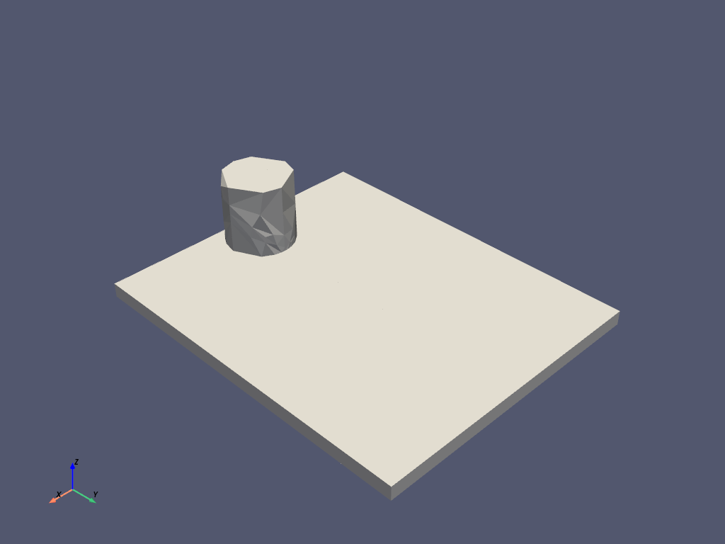
Figure 28.1: 3-D model of workpiece and tool
The FSW process generally requires a tool made of a harder material than the workpiece material being welded. In the past, FSW was used for soft workpiece materials such as aluminium. With the development of tools made from super-abrasive materials such as polycrystalline cubic boron nitride (PCBN), FSW has become possible with high-temperature materials such as stainless steel. A cylindrical PCBN tool is modeled in this case.
The workpiece sides parallel to the weld line are constrained in all the directions to simulate the clamping ends. The bottom side of the workpiece is constrained in the perpendicular (z) direction to simulate support at the bottom. Heat losses are considered on all the surfaces of the model. All 28.5. Boundary conditions and loading are symmetric across the weld centerline.
The simulation is performed in three load steps, each representing a respective phase ( 28.5.3. Loading) of the FSW process.
28.3. Modeling#
Modeling is a two-part task, as described in these topics:
28.3.1. Workpiece and tool modeling#
Two rectangular shaped plates (similar to those used in the reference model) are used as the workpiece. Dimensions have been reduced to decrease the simulation time.
The plate size is 3 x 1.25 x 0.125 in (76.2 x 31.75 x 3.18 mm). The tool shoulder diameter is 0.6 in (15.24 mm).
Plate thickness remains the same as that of the reference model, but the plate length and width are reduced. The plate width is reduced because the regions away from the weld line are not significantly affected by the welding process, and this example focuses primarily on the heat generation and temperature rise in the region nearest the weld line.
The height of the tool is equal to the shoulder diameter. Both the workpiece
(steel plates) and the tool are modeled using coupled-field element
SOLID226 with the structural-thermal option (KEYOPT(1)= 11).
# sphinx_gallery_thumbnail_path = '_static/tse28_setup.png'

import numpy as np
import pyvista

from ansys.mapdl.core import launch_mapdl
mapdl = launch_mapdl()
mapdl.prep7()

# ***** Problem parameters ********
l = 76.2e-03     # Length of each plate,m
w = 31.75e-03    # Width of each plate,m
t = 3.18e-03     # Thickness of each plate,m
r1 = 7.62e-03    # Shoulder radius of tool,m
h = 15.24e-03    # Height of tool, m
l1 = r1          # Starting location of tool on weldline
l2 = l-l1
tcc1 = 2e06      # Thermal contact conductance b/w plates,W/m^2'C
tcc2 = 10        # Thermal contact conductance b/w tool &
# workpiece,W/m^2'C
fwgt = 0.95      # weight factor for distribution of heat b/w tool
# & workpiece
fplw = 0.8       # Fraction of plastic work converted to heat
uz1 = t/4000     # Depth of penetration,m
nr1 = 3.141593*11  # No. of rotations in second load step
nr2 = 3.141593*45  # No. of rotations in third load step
uy1 = 60.96e-03  # Travelling distance along weld line
tsz = 0.01       # Time step size

# ==========================================================
# * Geometry
# ==========================================================
# * Node for pilot node
mapdl.n(1, 0, 0, h)
# * Workpiece geometry (two rectangular plates)
mapdl.block(0, w, -l1, l2, 0, -t)
mapdl.block(0, -w, -l1, l2, 0, -t)
# * Tool geometry
mapdl.cyl4(0, 0, r1, 0, r1, 90, h)
mapdl.cyl4(0, 0, r1, 90, r1, 180, h)
mapdl.cyl4(0, 0, r1, 180, r1, 270, h)
mapdl.cyl4(0, 0, r1, 270, r1, 360, h)
mapdl.vglue(3, 4, 5, 6)
A hexahedral mesh with dropped midside nodes is used because the presence of midside nodes (or quadratic interpolation functions) can lead to oscillations in the thermal solution, leading to nonphysical temperature distribution. A hexahedral mesh is used instead of a tetrahedral mesh to avoid mesh-orientation dependency. For more accurate results, a finer mesh is used in the weld-line region. The following figure shows the 3-D meshed model:
# ==========================================================
# * Meshing
# ==========================================================
mapdl.et(1, "SOLID226", 11)  # Coupled-field solid element,KEYOPT(1) is
# set to 11 for a structural-thermal analysis
mapdl.allsel()
mapdl.lsel("s", "", "", 4, 5)
mapdl.lsel("a", "", "", 14, 19, 5)
mapdl.lesize("all", "", "", 22, 5)
mapdl.lsel("s", "", "", 16, 17)
mapdl.lsel("a", "", "", 2, 7, 5)
mapdl.lesize("all", "", "", 22, "1/5")
mapdl.lsel("s", "", "", 1)
mapdl.lsel("a", "", "", 3)
mapdl.lsel("a", "", "", 6)
mapdl.lsel("a", "", "", 8)
mapdl.lsel("a", "", "", 13)
mapdl.lsel("a", "", "", 15)
mapdl.lsel("a", "", "", 18)
mapdl.lsel("a", "", "", 20)
mapdl.lesize("all", "", "", 44)
mapdl.lsel("s", "", "", 9, "")
mapdl.lsel("a", "", "", 22)
mapdl.lesize("all", "", "", 2)
mapdl.allsel("all")
mapdl.mshmid(2)  # midside nodes dropped
mapdl.vsweep(1)
mapdl.vsweep(2)
mapdl.vsel("u", "volume", "", 1, 2)
mapdl.mat(2)
mapdl.esize(0.0015)
mapdl.vsweep("all")
mapdl.allsel("all")

mapdl.eplot(vtk=True, background='white')
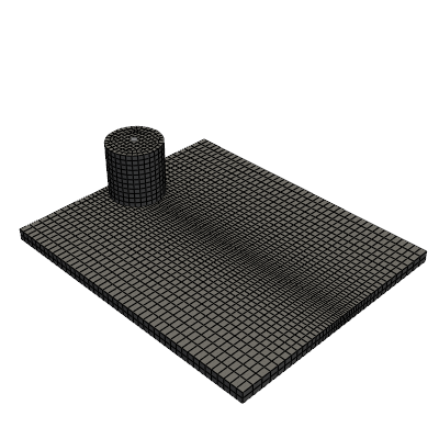
Figure 28.2: 3-D meshed model of workpiece and tool
28.3.2. Contact modeling#
Contact is modeled as follows for the FSW simulation:
Contact pair between the plates
Contact pair between tool and workpiece
Rigid surface constraint
28.3.2.1. Contact pair between the plates#
During the simulation, the surfaces to be joined come into contact. A standard
surface-to-surface contact pair using TARGE170 and CONTA174, as shown
in the following figure:
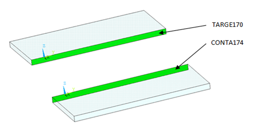
Fig. 20 Figure 28.3: Contact pair between plates#
The surface-projection-based contact method (KEYOPT(4) = 3 for contact
elements) is defined at the contact interface. The surface-projection-based
contact method is well suited to highly nonlinear problems that include
geometrical, material, and contact nonlinearities.
The problem simulates welding using the bonding capability of contact
elements. To achieve continuous bonding and simulate a perfect thermal contact
between the plates, a high thermal contact conductance (TCC) of 2 ⋅ 10E6 W/m2
°C is specified. (A small TCC value yields an imperfect contact and a
temperature discontinuity across the interface.) The conductance is specified
as a real constant for CONTA174 elements.
The maximum temperature ranges from 70 to 90 percent of the melting temperature
of the workpiece material. Welding occurs after the temperature of the material
around the contacting surfaces exceeds the bonding temperature (approximately
70 percent of the workpiece melting temperature). In this case, 1000 °C is
considered to be the bonding temperature based on the reference results. The
bonding temperature is specified using the real constant TBND for
CONTA174. When the temperature at the contact surface for closed contact
exceeds the bonding temperature, the contact type changes to bonded. The
contact status remains bonded for the remainder of the simulation, even though
the temperature subsequently decreases below the bonding value.
# * Define contact pair between two plates
mapdl.et(6, "TARGE170")
mapdl.et(7, "CONTA174")
mapdl.keyopt(7, 1, 1)  # Displacement & temp DOF
mapdl.keyopt(7, 4, 3)  # To include surface projection based method
mapdl.mat(1)
mapdl.asel("s", "", "", 5)
mapdl.nsla("", 1)
#mapdl.nplot()
mapdl.cm("tn.cnt", "node")  # Creating component on weld side of plate1

mapdl.asel("s", "", "", 12)
mapdl.nsla("", 1)
#mapdl.nplot()
mapdl.cm("tn.tgt", "node")  # Creating component on weld side of plate2

mapdl.allsel("all")
mapdl.type(6)
mapdl.r(6)
mapdl.rmodif(6, 14, tcc1)  # A real constant TCC, thermal contact
# conductance coeffi. b/w the plates, W/m^2'C
mapdl.rmodif(6, 35, 1000)  # A real constant TBND,Bonding temperature
# for welding, 'C
mapdl.real(6)
mapdl.cmsel("s", "tn.cnt")
mapdl.nplot(title='Example of contact nodes', background='white')
mapdl.esurf()
mapdl.type(7)
mapdl.real(6)
mapdl.cmsel("s", "tn.tgt")
mapdl.esurf()
mapdl.allsel("all")
28.3.2.2. Contact pair between tool and workpiece#
The tool plunges into the work piece, rotates, and moves along the weld line.
Because the frictional contact between the tool and workpiece is primarily
responsible for heat generation, a standard surface-to-surface contact pair is
defined between the tool and workpiece. The CONTA174 element is used to
model the contact surface on the top surface of the workpiece, and the
TARGE170 element is used for the tool, as shown in this figure:
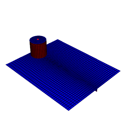
Figure 28.4: Contact pair between tool and workpiece.
CONTA174 in blue, and TARGE170 in red.
Two real constants are specified to model friction-induced heat generation.
The fraction of frictional dissipated energy converted into heat is modeled
first; the FHTG real constant is set to 1 to convert all frictional
dissipated energy into heat. The factor for the distribution of heat between
contact and target surfaces is defined next; the FWGT real constant is set
to 0.95, so that 95 percent of the heat generated from the friction flows into
the workpiece and only five percent flows into the tool.
A low TCC value (10 W/m2 °C) is specified for this contact pair because most of
the heat generated transfers to the workpiece. Some additional heat is also
generated by plastic deformation of the workpiece material. Because the
workpiece material softens and the value of friction coefficient drops as the
temperature increases, a variable coefficient of friction (0.4 to 0.2) is
defined (Mapdl.tb("FRIC") with
mapdl.tbtemp() and
Mapdl.tbdata()).
# * Define contact pair between tool & workpiece
mapdl.et(4, "TARGE170")
mapdl.et(5, "CONTA174")
mapdl.keyopt(5, 1, 1)  # Displacement & temp DOF
mapdl.keyopt(5, 5, 3)  # Close gap/reduce penetration with auto cnof
mapdl.keyopt(5, 9, 1)  # Exclude both initial penetration or gap
mapdl.keyopt(5, 10, 0)  # Contact stiffness update each iteration
# based

# Bottom & lateral(all except top) surfaces of tool for target
mapdl.vsel("u", "volume", "", 1, 2)
mapdl.allsel("below", "volume")
mapdl.nsel("r", "loc", "z", 0, h)
mapdl.nsel("u", "loc", "z", h)
mapdl.type(4)
mapdl.r(5)
mapdl.tb("fric", 5, 6)  # Definition of friction co efficient at
# different temp
mapdl.tbtemp(25)
mapdl.tbdata(1, 0.4)  # friction co-efficient at temp 25
mapdl.tbtemp(200)
mapdl.tbdata(1, 0.4)  # friction co-efficient at temp 200
mapdl.tbtemp(400)
mapdl.tbdata(1, 0.4)  # friction co-efficient at temp 400
mapdl.tbtemp(600)
mapdl.tbdata(1, 0.3)  # friction co-efficient at temp 600
mapdl.tbtemp(800)
mapdl.tbdata(1, 0.3)  # friction co-efficient at temp 800
mapdl.tbtemp(1000)
mapdl.tbdata(1, 0.2)  # friction co-efficient at temp 1000
mapdl.rmodif(5, 9, 500e6)  # Max.friction stress
mapdl.rmodif(5, 14, tcc2)  # Thermal contact conductance b/w tool and
# workpiece, 10 W/m^2'C
mapdl.rmodif(5, 15, 1)  # A real constant FHTG,the fraction of
# frictional dissipated energy converted
# into heat
mapdl.rmodif(5, 18, fwgt)  # A real constant FWGT, weight factor for
# the distribution of heat between the
# contact and target surfaces, 0.95
mapdl.real(5)
mapdl.mat(5)
mapdl.esln()
mapdl.esurf()
mapdl.allsel("all")
28.3.2.3. Rigid surface constraint#
The workpiece remains fixed in all stages of the simulation. The tool rotates
and moves along the weld line. A pilot node is created at the center of the top
surface of the tool in order to apply the rotation and translation on the tool.
The motion of the pilot node controls the motion of the entire tool. A rigid
surface constraint is defined between the pilot node (TARGE170) and the
nodes of the top surface of the tool (CONTA174). A multipoint constraint
(MPC) algorithm with contact surface behavior defined as bonded always is used
to constrain the contact nodes to the rigid body motion defined by the pilot
node.
The following contact settings are used for the CONTA174 elements:
To include MPC contact algorithm:
KEYOPT(2) = 2For a rigid surface constraint:
KEYOPT(4) = 2To set the behavior of contact surface as bonded (always):
KEYOPT(12) = 5
# * Define rigid surface constraint on tool top surface
mapdl.et(2, "TARGE170")
mapdl.keyopt(2, 2, 1)  # User defined boundary condition on rigid
# target nodes

mapdl.et(3, "CONTA174")
mapdl.keyopt(3, 1, 1)  # To include temp DOF
mapdl.keyopt(3, 2, 2)  # To include MPC contact algorithm
mapdl.keyopt(3, 4, 2)  # For a rigid surface constraint
mapdl.keyopt(3, 12, 5)  # To set the behavior of contact surface as a
# bonded (always)

mapdl.vsel("u", "volume", "", 1, 2)  # Selecting tool volume
mapdl.allsel("below", "volume")
mapdl.nsel("r", "loc", "z", h)  # Selecting nodes on the tool top surface
mapdl.type(3)
mapdl.r(3)
mapdl.real(3)
mapdl.esln()
mapdl.esurf()  # Create contact elements
mapdl.allsel("all")

# * Define pilot node at the top of the tool
mapdl.nsel("s", "node", "", 1)
mapdl.tshap("pilo")
mapdl.type(2)
mapdl.real(3)
mapdl.e(1)  # Create target element on pilot node
mapdl.allsel()

# Top surfaces of plates nodes for contact
mapdl.vsel("s", "volume", "", 1, 2)
mapdl.allsel("below", "volume")
mapdl.nsel("r", "loc", "z", 0)
mapdl.type(5)
mapdl.real(5)
mapdl.esln()
mapdl.esurf()
mapdl.allsel("all")
[82, 87, 110]
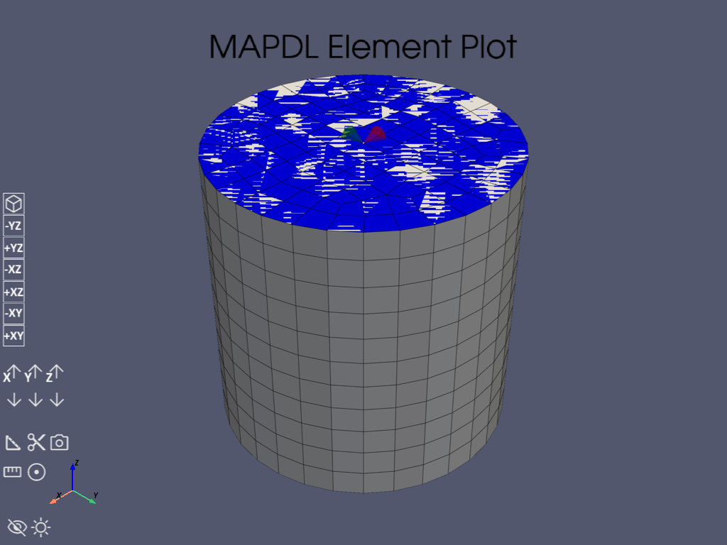
Figure 28.5: Rigid surface constrained. Pilot node or master with applied boundary conditions and the constrained top surface of the tool (blue).**
28.4. Material properties#
Accurate temperature calculation is critical to the FSW process because the stresses and strains developed in the weld are temperature-dependent. Thermal properties of the 304L steel plates such as thermal conductivity, specific heat, and density are temperature-dependent. Mechanical properties of the plates such as Young’s modulus and the coefficient of thermal expansion are considered to be constant due to the limitations of data available in the literature.
It is assumed that the plastic deformation of the material uses the Von Misses
yield criterion, as well as the associated flow rule and the work-hardening
rule. Therefore, a bilinear isotropic hardening model (TB,PLASTIC,,,,BISO)
is selected.
The following table shows the material properties of the workpiece:
Table 28.1: Workpiece material properties
Property |
Value |
|---|---|
Linear properties |
|
Young’s modulus |
193 GPa |
Poisson’s ratio |
0.3 |
Coefficient of thermal expansion |
18.7 µm/m °C |
Bilinear isotropic hardening constants (``TB,PLASTIC,,,,BISO``) |
|
Yield stress |
290 MPa |
Tangent modulus |
2.8 GPa |
Temperature-dependent material properties |
|
Temperature (°C) |
0 |
Thermal conductivity (W/m °C) |
16 |
Specific heat (J/Kg °C) |
500 |
Density (Kg/m3) |
7894 |
Mapdl.tbdata()
defines the yield stress and tangent modulus.
The fraction of the plastic work dissipated as heat during FSW is about 80
percent. Therefore, the fraction of plastic work converted to heat
(Taylor-Quinney coefficient) is set to 0.8 (Mapdl.mp("QRATE")) for the calculation of plastic heat generation in
the workpiece material.
To weld a high-temperature material such as 304L stainless steel, a tool composed of hard material is required. Tools made from super-abrasive materials such as PCBN are suitable for such processes, and so a cylindrical PCBN tool is used here. The material properties of the PCBN tool are obtained from the references: [Ozel2008] and [Mishra2007].
The following table shows the material properties of the PCBN tool:
Table 28.2: Material properties of the PCBN tool
Property |
Value |
|---|---|
Young modulus |
680 GPa |
Poisson’s ratio |
0.22 |
Thermal conductivity |
100 W/m °C |
Specific heat |
750 J/Kg °C |
Density |
4280 Kg/m3 |
The following code setup the material properties:
# ==========================================================
# * Material properties
# ==========================================================
# * Material properties for 304l stainless steel Plates
mapdl.mp("ex", 1, 193e9)  # Elastic modulus (N/m^2)
mapdl.mp("nuxy", 1, 0.3)  # Poisson's ratio
mapdl.mp("alpx", 1, 1.875e-5)  # Coefficient of thermal expansion, µm/m'c
# Fraction of plastic work converted to heat, 80%
mapdl.mp("qrate", 1, fplw)

# *BISO material model
EX = 193e9
ET = 2.8e9
EP = EX*ET/(EX-ET)
mapdl.tb("plas", 1, 1, "", "biso")  # Bilinear isotropic material
mapdl.tbdata(1, 290e6, EP)  # Yield stress & plastic tangent modulus
mapdl.mptemp(1, 0, 200, 400, 600, 800, 1000)
mapdl.mpdata("kxx", 1, 1, 16, 19, 21, 24, 29, 30)  # therm cond.(W/m'C)
mapdl.mpdata("c", 1, 1, 500, 540, 560, 590, 600, 610)  # spec heat(J/kg'C)
mapdl.mpdata("dens", 1, 1, 7894, 7744, 7631, 7518, 7406, 7406)  # kg/m^3

# * Material properties for PCBN tool
mapdl.mp("ex", 2, 680e9)  # Elastic modulus (N/m^2)
mapdl.mp("nuxy", 2, 0.22)  # Poisson's ratio
mapdl.mp("kxx", 2, 100)  # Thermal conductivity(W/m'C)
mapdl.mp("c", 2, 750)  # Specific heat(J/kg'C)
mapdl.mp("dens", 2, 4280)  # Density,kg/m^3
28.5. Boundary conditions and loading#
This section describes the thermal and mechanical boundary conditions imposed on the FSW model:
28.5.1. Thermal boundary conditions#
The frictional and plastic heat generated during the FSW process propagates rapidly into remote regions of the plates. On the top and side surfaces of the workpiece, convection and radiation account for heat loss to the ambient. Conduction losses also occur from the bottom surface of the workpiece to the backing plate.
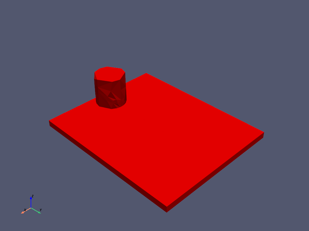

Figure 28.6: Thermal boundary conditions. Convection loads (red) and conduction loads (yellow)
Available data suggest that the value of the convection coefficient lies between 10 and 30 W/m2 °C for the workpiece surfaces, except for the bottom surface. The value of the convection coefficient is 30 W/m2°C for workpiece and tool. This coefficient affects the output temperature. A lower coefficient increases the output temperature of the model. A high overall heat-transfer coefficient (about 10 times the convective coefficient) of 300 W/m2 °C is assumed for the conductive heat loss through the bottom surface of the workpiece. As a result, the bottom surface of the workpiece is also treated as a convection surface for modeling conduction losses. Because the percentage of heat lost due to radiation is low, radiation heat losses are ignored. An initial temperature of 25 °C is applied on the model. Temperature boundary conditions are not imposed anywhere on the model.
# Initial boundary conditions.
mapdl.tref(25)  # Reference temperature 25'C
mapdl.allsel()
mapdl.nsel("all")
mapdl.ic("all", "temp", 25)  # Initial condition at nodes,temp 25'C


# Thermal boundary conditions
# Convection heat loss from the workpiece surfaces
mapdl.vsel("s", "volume", "", 1, 2)  # Selecting the workpiece
mapdl.allsel("below", "volume")
mapdl.nsel("r", "loc", "z", 0)
mapdl.nsel("a", "loc", "x", -w)
mapdl.nsel("a", "loc", "x", w)
mapdl.nsel("a", "loc", "y", -l1)
mapdl.nsel("a", "loc", "y", l2)
mapdl.sf("all", "conv", 30, 25)

# Convection (high)heat loss from the workpiece bottom
mapdl.nsel("s", "loc", "z", -t)
mapdl.sf("all", "conv", 300, 25)
mapdl.allsel("all")

# Convection heat loss from the tool surfaces
mapdl.vsel("u", "volume", "", 1, 2)  # Selecting the tool
mapdl.allsel("below", "volume")
mapdl.csys(1)
mapdl.nsel("r", "loc", "x", r1)
mapdl.nsel("a", "loc", "z", h)
mapdl.sf("all", "conv", 30, 25)
mapdl.allsel("all")

# Constraining all DOFs at pilot node except the temp DOF
mapdl.d(1, "all")
mapdl.ddele(1, "temp")
mapdl.allsel("all")
28.5.2. Mechanical boundary conditions#
The workpiece is fixed by clamping each plate. The clamped portions of the plates are constrained in all directions. To simulate support at the bottom of the plates, all bottom nodes of the workpiece are constrained in the perpendicular direction (z direction).
[82, 87, 110]
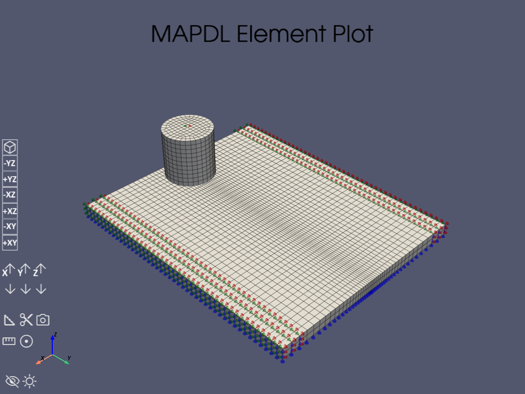
Figure 28.7: Mechanical boundary conditions:
X-direction (UX) in red, Y-direction (UY) in green, and Z-direction (UZ) in blue.
# Mechanical boundary conditions
# 20% ends of the each plate is constraint
mapdl.nsel("s", "loc", "x", -0.8*w, -w)
mapdl.nsel("a", "loc", "x", 0.8*w, w)
mapdl.d("all", "uz", 0)  # Displacement constraint in x-direction
mapdl.d("all", "uy", 0)  # Displacement constraint in y-direction
mapdl.d("all", "ux", 0)  # Displacement constraint in z-direction
mapdl.allsel("all")

# Bottom of workpiece is constraint in z-direction
mapdl.nsel("s", "loc", "z", -t)
mapdl.d("all", "uz")  # Displacement constraint in z-direction
mapdl.allsel("all")
28.5.3. Loading#
The FSW process consists of three primary phases:
Plunge – The tool plunges slowly into the workpiece
Dwell – Friction between the rotating tool and workpiece generates heat at the initial tool position until the workpiece temperature reaches the value required for the welding.
Traverse (or Traveling) – The rotating tool moves along the weld line.
During the traverse phase, the temperature at the weld line region rises, but the maximum temperature values do not surpass the melting temperature of the workpiece material. As the temperature drops, a solid continuous joint appears between the two plates.
For illustrative purposes, each phase of the FSW process is considered a separate load step. A rigid surface constraint is already defined for applying loading on the tool.
The following table shows the details for each load step.
Table 28.3: Load steps
Load step |
Time period (sec) |
Loadings on pilot node |
Boundary condition |
|---|---|---|---|
1 |
1 |
Displacement boundary condition |
|
2 |
5.5 |
Rotational boundary condition |
|
3 |
22.5 |
Displacement and rotational boundary conditions together on the pilot node |
|
The tool plunges into the workpiece at a very shallow depth, then rotates to generate heat. The depth and rotating speeds are the critical parameters for the weld temperatures. The parameters are determined based on the experimental data of Zhu and Chao [Zhu2004]. The tool travels from one end of the welding line to the other at a speed of 2.7 mm/s.
28.6. Analysis and solution controls#
A nonlinear transient analysis is performed in three load steps using
structural-thermal options of SOLID226 and
CONTA174.
FSW simulation includes factors such as nonlinearity, contact, friction, large plastic deformation, structural-thermal coupling, and different loadings at each load step. The solution settings applied consider all of these factors.
The first load step in the solution process converges within a few substeps, but the second and third load steps converge only after applying the proper solution settings shown in the following table:
Table 28.4: Solution settings
Solution setting |
Description of setting and comments |
|---|---|
|
Transient analysis. |
|
For contact problems,this option is useful for enhancing convergence. |
|
Controls the time-step cutback during a nonlinear solution and specifies the maximum equivalent plastic strain allowed within a time-step. If the calculated value exceeds the specified value, the program performs a cutback (bisection). |
|
Includes large-deflection effects or large strain effects, according to the element type. |
|
Recommended for contact elements with high friction coefficients. |
|
To speed up convergence in a coupled-field transient analysis, the structural dynamic effects are turned off. These structural effects are not important in the modeling of heat generation due to friction; however,the thermal dynamic effects are considered here. |
|
The loads applied to intermediate substeps within the load step are ramped because the structural dynamic effects are set to off. |
To allow for a faster solution, automatic time-stepping is activated
(Mapdl.autots("on")). The initial time
step size (Mapdl.deltim()) is set to
0.1, and the minimum time step is set to 0.001. The maximum time step is set as
0.2 in load steps 2 and 3. A higher maximum time-step size may result in an
unconverged solution.
The time step values are determined based on mesh or element size. For stability, no time-step limitation exists for the implicit integration algorithm. Because this problem is inherently nonlinear and an accurate solution is necessary, a disturbance must not propagate to more than one element in a time step; therefore, an upper limit on the time step size is required. It is important to choose a time step size that does not violate the subsequent criterion (minimum element size, maximum thermal conductivity over the whole model, minimum density, and minimum specific heat).
mapdl.solu()
mapdl.antype(4)  # Transient analysis
mapdl.lnsrch('on')
mapdl.cutcontrol('plslimit', 0.15)
mapdl.kbc(0)  # Ramped loading within a load step
mapdl.nlgeom("on")  # Turn on large deformation effects
mapdl.timint("off", "struc")  # Structural dynamic effects are turned off.
mapdl.nropt('unsym')

## Solving
# Load step1
mapdl.time(1)
mapdl.nsubst(10, 1000, 10)
mapdl.d(1, "uz", -uz1)  # Tool plunges into the workpiece
mapdl.outres("all", "all")
mapdl.allsel()
mapdl.solve()
mapdl.save()

# Load step2
mapdl.time(6.5)
mapdl.d(1, "rotz", nr1)  # Rotation of tool, 60rpm
mapdl.deltim(tsz, 0.001, 0.2)
mapdl.outres("all", 10)
mapdl.allsel()
mapdl.solve()
mapdl.save()

# Load step3
mapdl.time(29)
mapdl.d(1, "rotz", nr2)  # Rotation of tool,60rpm
mapdl.d(1, "uy", uy1)  # Displacement of tool along weldline
mapdl.deltim(tsz, 0.001, 0.2)
mapdl.outres("all", 10)
mapdl.solve()
mapdl.finish()
mapdl.save()
28.7. Results and discussion#
The following results topics for the FSW simulation are available:
28.7.1. Deformation and stresses#
It is important to observe the change in various quantities around the weld line during the FSW process. The following figure shows the deflection of the workpiece due to plunging of the tool in the first load step:
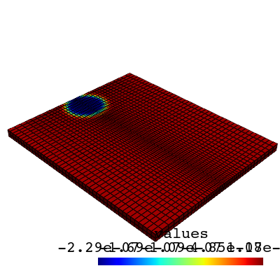
Figure 28.9: Deflection at workpiece after load step 1
The deflection causes high stresses to develop on the workpiece beneath the tool, as shown in this figure:
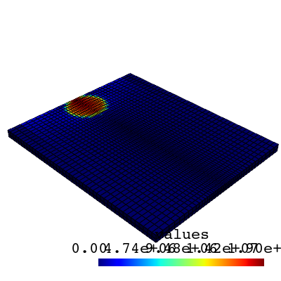
Figure 28.10: Von Mises stress after load step 1
Following load step 1, the temperature remains unchanged (25 °C), as shown in this figure:
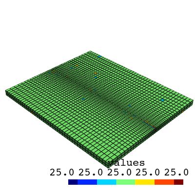
Figure 28.11: Temperature after load step 1
As the tool begins to rotate at this location, the frictional stresses develop and increase rapidly. The following two figures show the increment in contact frictional stresses from load step 1 to load step 2:
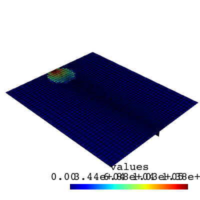
Figure 28.12: Frictional stress after load step 1

Figure 28.13: Frictional stress after load step 2
All frictional dissipated energy is converted into heat during load step 2. The heat is generated at the tool-workpiece interface. Most of the heat is transferred to the workpiece (FWGT is specified to 0.95). As a result, the temperature of the workpiece increases rapidly compared to that of the tool.
28.7.2. Temperature results#
The following two figures shows the temperature rise due to heat generation in the second and third load steps:
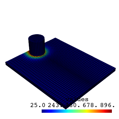
Figure 28.14: Temperature after load step 2
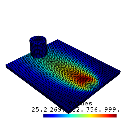
Figure 28.15: Temperature after load step 3
The maximum temperature on the workpiece occurs beneath the tool during the last two load steps. Heat generation is due to the mechanical loads. No external heat sources are used. As the temperature increases, the material softens and the coefficient of friction decreases. A temperature-dependent coefficient of friction (0.4 to 0.2) helps to prevent the maximum temperature from exceeding the material melting point.
The observed temperature rise in the model shows that heat generation during the second and third load steps is due to friction between the tool shoulder and workpiece, as well as plastic deformation of the workpiece material.
The melting temperature of 304L stainless steel is 1450 °C. As shown in the following figure, the maximum temperature range at the weld line region on the workpiece beneath the tool is well below the melting temperature of the workpiece material during the second and third load steps, but above 70 percent of the melting temperature:
Figure 28.16: Maximum temperature (on workpiece beneath the tool) variation with time
The two plates can be welded together within this temperature range.
The following figure shows the temperature distributions on the top surface of the workpiece along the transverse distance (perpendicular to the weld line):
Figure 28.17: Temperature distribution on the top surface of workpiece at various locations
As shown in the following figure and table, the temperature plots indicate the temperature distribution at various locations on the weld line when the maximum temperature occurs at those locations:
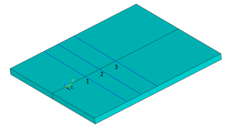
Fig. 21 Figure 28.18: Various locations on the workpiece#
Table 28.5: Locations on weld line
Location number |
Distance on the weld line in y direction |
Time when maximum temperature occurs |
|---|---|---|
1 |
0.016 m |
15.25 Sec |
2 |
0.027 m |
19.2 Sec |
3 |
0.040 m |
24 Sec |
The following figure shows the temperature distribution in the thickness direction at location 1:
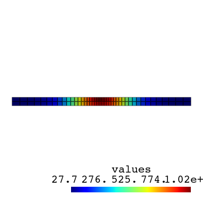
Figure 28.19: Temperature distribution in thickness direction at location 1
As expected, the highest temperature caused by heat generation appears around the weld line region. By comparing the above temperature results with the reference results, it can be determined that the temperatures obtained at the weld line are well below the melting temperature of the workpiece material, but still sufficient for friction stir welding.
The following table and figure show the time-history response of the temperature at various locations on the weld line:
Location number |
Distance on the weld line |
|---|---|
1 |
0.018 m |
2 |
0.023 m |
3 |
0.027 m |
4 |
0.032 m |
5 |
0.035 m |
6 |
0.039 m |
Figure 28.20: Temperature variation with time on various joint locations
28.7.3. Welding results#
A bonding temperature of 1000 °C is already defined for the welding simulation at the interface of the plates. The contact status at this interface after the last load step is shown in the following figure:
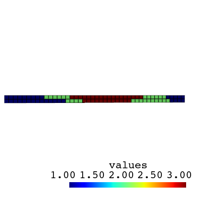
Figure 28.21: Contact status at interface with bonding temperature 1000 °C Elements can be in near-contact (blue), sliding (green) or sticking (red) states.
The sticking portion of the interface shows the bonding or welding region of the plates. If the bonding temperature was assumed to be 900 °C, then the welding region would increase, as shown in this figure:
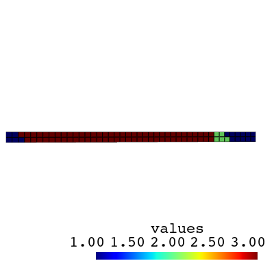
Figure 28.22: Contact status at interface with bonding temperature 900 °C Elements can be in near-contact (blue), sliding (green) or sticking (red) states.
28.7.4. Heat generation#
Friction and plastic deformation generate heat. A calculation of frictional and plastic heat generation is performed. The generation of heat due to friction begins in the second load step.
The CONTA174 element’s FDDIS (SMISC item) output option is used to
calculate frictional heat generation on the workpiece. This option gives the
frictional energy dissipation per unit area for an element. After multiplying
this value with the corresponding element area, the friction heat-generation
rate for an element is calculated. By summing the values from each CONTA174
element of the workpiece, the total frictional heat generation rate is
calculated for a given time.
It is possible to calculate the total frictional heat-generation rate at each
time-step (Mapdl.etable). The
following figure shows the plot of total frictional heat generation rate on the
workpiece with time:
Figure 28.23: Total frictional heat rate variation with time
The plot indicates that the frictional heat starts from the second load step (after 1 second).
The element contact area can be calculated using the
CONTA174 element CAREA (NMISC, 58) output
option.
mapdl.post1()
mapdl.set("last")
nst = mapdl.get_value("nst", "active", "", "set", "nset")  # To get number of data sets on result file

# Total frictional heat rate
mapdl.esel("s", "real", "", 5)
mapdl.esel("r", "ename", "", 174)  # Selecting the contact elements on Workpiece
fht = np.zeros(nst)
for i in range(1, nst):
    mapdl.set("", "", "", "", "", "", i)

    # Frictional energy dissipation per unit
    # area for an element, FDDIS
    mapdl.etable("fri", "smisc", 18)
    mapdl.etable("are1", "nmisc", 58)  # Area of each contact element

    # Multiplying frictional energy dissipation
    # per unit area with the area of
    # corresponding element
    mapdl.smult("frri", "fri", "are1")
    mapdl.ssum()  # Summing up the Frictional heat rate

    # Total frictional heat rate on
    # workpiece at a particular time
    frhi = mapdl.get('frhi', 'ssum',, 'item', 'frri')
    fht(i) = frhi

mapdl.parsav("all")
mapdl.allsel("all")
mapdl.finish()

mapdl.post26()
mapdl.file("fsw", "rst")
mapdl.numvar(200)
mapdl.solu(191, "ncmit")  # Solution summary data per substep to be
# stored for cumulative no. of iterations.
mapdl.store("merge")  # Merge data from results file
mapdl.filldata(191, "", "", "", 1, 1)
mapdl.realvar(191, 191)
mapdl.parres("new", "fsw", "parm")
mapdl.vput("fht", 11, "", "", "fric_heat")
mapdl.plvar(11)  # Plot of frictional heat rate against time
A similar calculation is performed to check the heat generation from plastic
deformation on the workpiece. The SOLID226 element’s output option
PHEAT (NMISC, 5) gives the plastic heat generation rate per unit
volume. After multiplying this value with the corresponding element volume,
the plastic heat generation rate for an element is calculated. By summing the
values from each element (SOLID226) of the workpiece, the total plastic
heat generation rate is calculated for a particular time.
It is possible to calculate the total frictional heat generation rate at each
time-step (Mapdl.etable). The following
figure shows the plot of the total plastic heat-generation rate with time.
Figure 28.24: Total plastic heat rate variation with time
mapdl.post1()
mapdl.set("last")
nst = mapdl.get("nst", "active", "", "set", "nset")  # To get number of data sets on result file

# Total plastic heat rate
mapdl.esel("s", "mat", "", 1)  # Selecting the coupled elements on workpiece
mapdl.etable("vlm1", "volu")  # Volume of the each element
pha = np.zeros(nst)

for i in range(1, nst):
    mapdl.set("", "", "", "", "", "", i)

    # Plastic heat rate per unit volume on
    # each element, PHEAT
    mapdl.etable("pi", "nmisc", 5)

    # Multiplying plastic heat rate per unit
    # volume with the volume of
    # corresponding element
    mapdl.smult("psi", "pi", "vlm1")

    mapdl.ssum()  # Summing up the plastic heat rate
    # Total plastic heat rate on workpiece
    # at a particular time
    ppi = mapdl.get('ppi','ssum',,'item','psi')

    pha[i] = ppi

mapdl.parsav("all")
mapdl.allsel("all")

mapdl.post26()
mapdl.file("fsw", "rst")
mapdl.numvar(200)

# solution summary data per substep to be
# stored for cumulative no. of iterations.
mapdl.solu(191, "ncmit")
mapdl.store("merge")  # Merge data from results file
mapdl.filldata(191, "", "", "", 1, 1)
mapdl.realvar(191, 191)
mapdl.parres("new", "fsw", "parm")
mapdl.vput("pha", 10, "", "", "pheat_nmisc")
mapdl.plvar(10)  # Plot of Plastic heat rate against time
Figure 28.23 and Figure 28.24 show that friction is responsible for generating most of the heat needed, while the contribution of heat due to plastic deformation is less significant. Because the tool-penetration is shallow and the tool pin is ignored, the plastic heat is small compared to frictional heat.
28.8. Exit MAPDL#
mapdl.finish()
mapdl.exit()
28.9. Recommendations#
To perform a similar FSW analysis, consider the following hints and recommendations:
FSW is a coupled-field (structural-thermal) process. The temperature field affects the stress distribution during the entire process. Also, heat generated in structural deformation affects the temperature field. The direct method of coupling is recommended for such processes. This method involves just one analysis that uses a coupled-field element containing all necessary degrees of freedom. Direct coupling is advantageous when the coupled-field interaction involves strongly coupled physics or is highly nonlinear.
A nonlinear transient analysis is preferable for simulations where the objective is to study the transient temperature and transient heat transfer.
The dynamic effects of different physics should be controlled. In this problem, for example, the dynamic effects of the structural degrees of freedom are disabled as they are unimportant.
Separating the solution process into three load steps helps you to understand the physics and solve the problem.
The contact between the two plates must be nearly perfect to maintain temperature continuity. For a perfect thermal contact, specify a high thermal contact conductance (TCC) coefficient between workpiece plates. A high coefficient results in temperature continuity across the interface.
Because the problem is nonlinear, proper solution settings are required. Set the following analysis controls to the appropriate values to achieve the converged solution:
Mapdl.lnsrch(),Mapdl.cutcontrol(),Mapdl.kbc(),Mapdl.neqit(),Mapdl.nropt(), andMapdl.autots().Convergence at the second and third load steps is difficult to achieve. The depth of penetration of the tool on the workpiece (
UZ), rotational speed of the tool (ROTZ), and time-step size play crucial roles in the convergence of the second load step. Use a very small time-step size if the rotational speed is higher than 60 RPM.A symmetric mesh (about the joint line) is preferred to capture the exact outputs and their effects on the workpiece. A hex mesh with dropped midside nodes is recommended for the workpiece as well as the tool. This approach helps to maintain symmetry and prevent the temperature from reaching negative values during the simulation.
A minimum of two element layers is required in the thickness direction. A fine sweep mesh near the weld line yields more accurate results; however, too fine a mesh increases computational time. A fine mesh is unnecessary on the tool side. To minimize computational time, the tool can be considered to be rigid with no temperature degrees of freedom.
28.10. References#
The following papers are cited in this example problem:
Zhu, X. K. & Chao, Y. J. (2004). Numerical simulation of transient temperature and residual stresses in friction stir welding of 304L stainless steel. Journal of Materials Processing Technology. 146(2), 263-272.
Prasanna, P., Rao, B. S., & Rao, G. K. (2010). Finite element modeling for maximum temperature in friction stir welding and its validation. Journal of Advanced Manufacturing Technology. 51, 925-933.
Ozel, T., Karpat, Y., & Srivastava, A. (2008). Hard turning with variable micro-geometry PcBN tools. CIRP Annals - Manufacturing Technology. 57, 73-76.
Mishra, R. S. (2007). Friction Stir Welding and Processing. Ed. R. S. Mishra and M. W. Mahoney. Materials Park, OH: ASM International.
28.11. Input files#
The following files were used in this problem:
fsw.cdb– Common database file containing the FSW model information
For more information, see Obtaining the input files.