Inverse-solving analysis of a cardiovascular structure#
This example problem demonstrates the capabilities and advantages of using a nonlinear static analysis with inverse solving to investigate the biomechanics of a cardiovascular system.
The following topics are available:
This example is inspired from the model and analysis defined in Chapter 62 of the Mechanical APDL technology showcase manual.
1. Introduction#
Finite element models of cardiovascular system components (such as the heart valve or blood vessels) are based on in vivo organ geometries obtained from 3D imaging systems such as computed tomography (CT) or magnetic resonance imaging (MRI).
Although medical imaging techniques offer accurate in vivo visualization of 3D patient-specific geometries, the geometries are under a loaded state (for example, in the presence of blood pressure) and lack in vivo stress/strain field information. Therefore, a nonlinear analysis performed directly on the geometry to simulate additional loading leads to inaccurate results.
In such cases, an inverse-solving analysis uses input geometry consisting of images where the models are already in a deformed shape under applied loads. The material properties and applied loads are known. The analysis can then determine the following:
The organ geometries at zero-pressure state (zero-pressure configuration)
The stress and strain fields on the in vivo organ geometries (the input geometries)
The behavior and response of the organ geometries when increasing the loading and taking accounting for prestressed effects
1.1. Problem description#
A mouse-specific 3D geometry of the aortic lumen containing four side branches is considered:
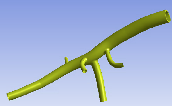
The model represents an approximated geometry of the abdominal aorta of a mouse, based on the reference.[1] The geometry is considered at end-diastolic pressure (80 mm Hg). The purpose of the analysis is to solve for end-systolic pressure (120 mm Hg).
This figure shows the inner diameter of the model at various approximate locations:
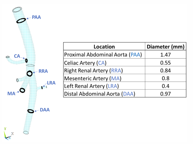
The wall thickness is assumed to be 20 percent of the local radius, so it varies throughout the structure.
1.2. Starting MAPDL as a service#
  # Starting MAPDL as a service and importing an external model
  from ansys.mapdl.core import launch_mapdl
  from ansys.mapdl.core.examples.downloads import download_tech_demo_data

  # Start MAPDL as a service
  mapdl = launch_mapdl(loglevel="WARNING", print_com=True)
  print(mapdl)

.. code-block:: none

   Mapdl
   -----
   PyMAPDL Version:     0.70.2
   Interface:           grpc
   Product:             Ansys Mechanical Enterprise
   MAPDL Version:       25.1
   Running on:          localhost
                        (127.0.0.1)
2. Setting up the model#
The model is meshed mostly with the higher-order hexahedral SOLID186 elements (about 99.4 percent of the total mesh), as shown in the following figure. However, it also has relatively a small number of tetrahedral SOLID187 elements (about 0.6 percent of the total mesh).
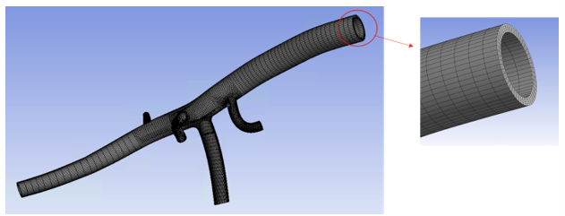
The mesh consists of 62123 elements with 4 elements to represent the wall thickness and at least 52 elements (or more) in the circumferential direction at most locations. Mixed u-P element formulation is enabled (KEYOPT(6) = 1).
# Starting MAPDL as a service and importing an external model
from ansys.mapdl.core import launch_mapdl
from ansys.mapdl.core.examples.downloads import download_tech_demo_data
mapdl = launch_mapdl()
# Download the CDB file of aortic lumen.
aorta_mesh_file = download_tech_demo_data(
"td-62", "inverse_analysis_cardiovascular_structure.cdb"
)
# Entering the PREP7 processor in MAPDL instance.
mapdl.clear()
mapdl.prep7()
# Reads a CDB file of solid model and database information into the database.
mapdl.cdread("comb", fname = aorta_mesh_file)
# Selects all entities with a single command.
mapdl.allsel("all", "all")
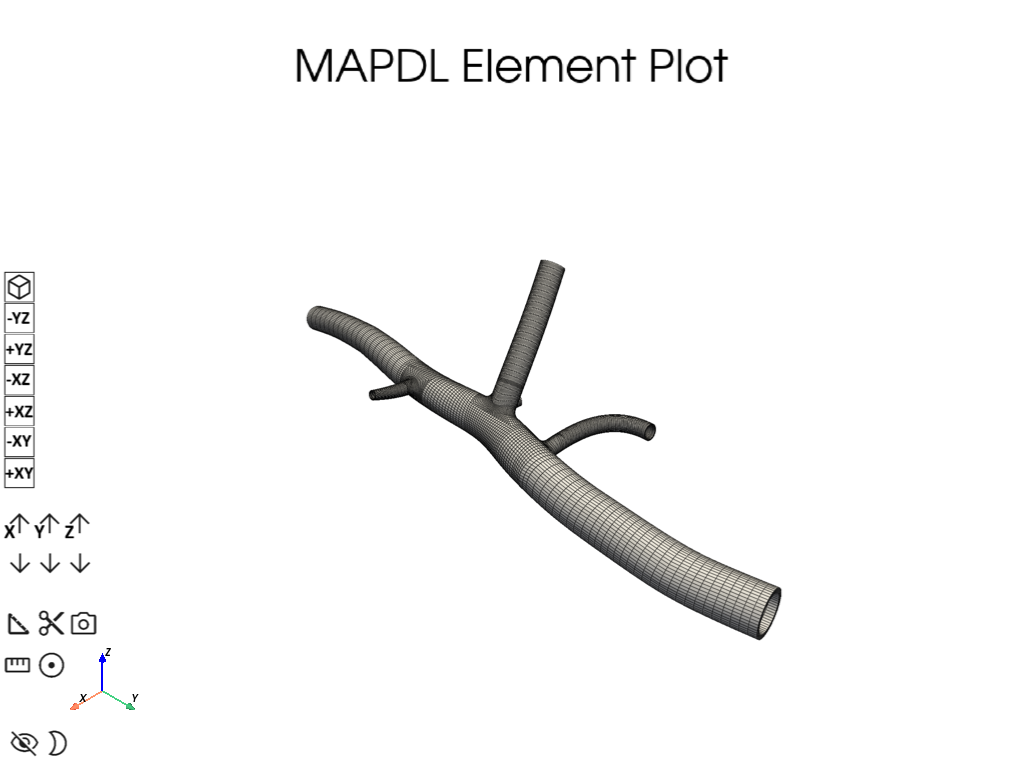
# Element plot of the Abdominal Aorta Model
mapdl.eplot(background='w', theme=mytheme, notebook=True, jupyter_backend='html')
# Exits from a pre-processor.
mapdl.finish()
# Exists MAPDL instance.
mapdl.exit()
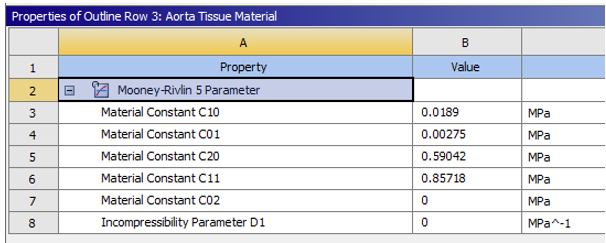
2.1. Material properties#
A Mooney-Rivlin hyperelastic material model with the following constants [4] is used to model the abdominal aorta:
2.2. Boundary conditions and loading#
The free radial boundary conditions are applied at each end cross-section in the model:
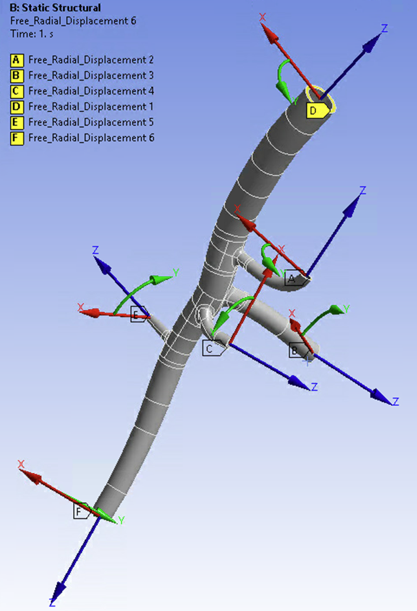
Local cylindrical coordinate systems are created at each end cross-section. The nodes in each end cross-section are constrained in all degrees of freedom except for the respective local radial direction.
A uniformly-distributed pressure load is applied on the inner surfaces of the model.
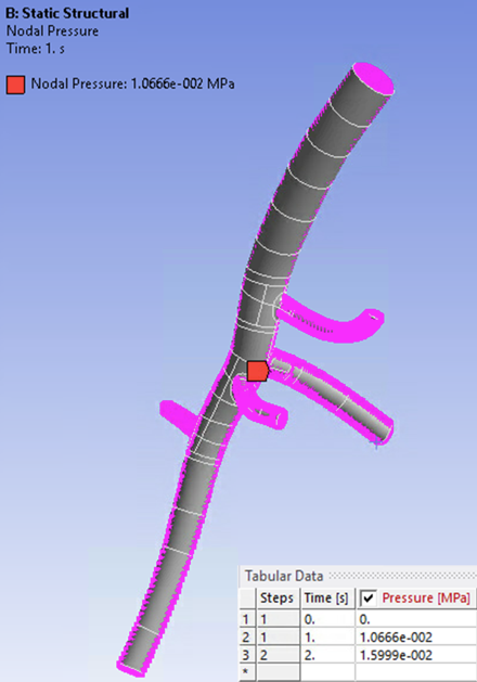
Because the input geometry is considered at end-diastolic pressure, a pressure load of 80 mm Hg (1.0666e-02 MPa) is applied on the inner surfaces of the model in the first load step (inverse-solving). The pressure is increased to 120 mm Hg (1.5999e-02 MPa) in the second load step (forward-solving).
3. Analysis#
The analysis for this problem is performed in two load steps:
3.1. Load step 1 (inverse-solving)#
Load step 1 (inverse-solving) - A nonlinear static analysis with inverse solving (INVOPT,ON) is performed on the input geometry of the model (at end-diastolic pressure (80 mm Hg)) to determine the zero-pressure geometry of the model and to obtain the stress/strain results on the input geometry.
# Enter solution processor and specify solution controls.
mapdl.slashsolu()
# Define the analysis type as static.
mapdl.antype(0)
# Turn on large deflection effects.
mapdl.nlgeom("on")
# Define "Sparse" solver option.
mapdl.eqslv("sparse", keepfile="1")

mapdl.cntr("print", 1)          # Print convergence control information
mapdl.dmpoption("emat", "no")   # Don't combine emat file for DANSYS
mapdl.dmpoption("esav", "no")   # Don't combine esav file for DANSYS

# Turn on "inverse-solving" option for Initial Steps.
mapdl.run("invopt,on")

# Controls file writing for multiframe restarts.
mapdl.nldiag("cont", "iter")
mapdl.rescontrol("define", "last", "last", "", "dele")

# Specify surface "pressures" loads.
mapdl.esel("u", "ename", "", 153, 156)
mapdl.sf("_CM968PRES", "pres", "%_loadvari968 %")
mapdl.esel("all")
mapdl.nopr()
mapdl.gopr()

# Turned on automatic time stepping.
mapdl.autots("on")

# Specifies the number of substeps to be taken this load step.
# Note: Please be aware that the number of substeps is decreased to reduce the computational effort.
#mapdl.nsubst(nsbstp='10', nsbmx='1000', nsbmn='5', carry="OFF")
mapdl.nsubst(nsbstp='2', nsbmx='2', nsbmn='2', carry="OFF")

# Sets the time for a first load step.
mapdl.time(time='1.0')

# Controls the solution data written to the database.
mapdl.outres("erase")
mapdl.outres("all", "none")
mapdl.outres("nsol", "all")
mapdl.outres("rsol", "all")
mapdl.outres("eangl", "all")
mapdl.outres("etmp", "all")
mapdl.outres("veng", "all")
mapdl.outres("strs", "all")
mapdl.outres("epel", "all")
mapdl.outres("eppl", "all")
mapdl.outres("cont", "all")

# Solve the load step 1 (inverse-solving).
mapdl.solve()
3.2. Load step 2 (forward-solving)#
After an inverse-solving load step, the solver generally allows an analysis to continue as forward-solving in a new load step. You can modify existing loads or apply new loads in the forward-solving step. For more information, see Reverting to forward solving and continuing the analysis as a new load step in the Structural Analysis Guide.
Load step 2 (forward-solving) - To solve the model for end-systolic pressure (120 mm Hg), the solution continues using forward solving (INVOPT,OFF). The pressure load is increased from 80 mm Hg to 120 mm Hg. Continuing the solution as a new load step following the inverse-solving load step eliminates a step in the simulation, allowing for a more efficient analysis.
# Solution Control for the load step 2 (forward-solving).

# Turned on automatic time stepping.
mapdl.autots("on")

# Specifies the number of substeps to be taken this load step.
# Note: Please be aware that the number of substeps is decreased to reduce the computational effort.
#mapdl.nsubst(nsbstp='10', nsbmx='1000', nsbmn='5', carry="OFF")
mapdl.nsubst(nsbstp='2', nsbmx='2', nsbmn='2', carry="OFF")

# Sets the time for the second load step.
mapdl.time(time='2.0')

# Turn off "inverse-solving" option for the second steps.
mapdl.run("invopt,off")

# Controls the solution data written to the database.
mapdl.outres("erase")
mapdl.outres("all", "none")
mapdl.outres("nsol", "all")
mapdl.outres("rsol", "all")
mapdl.outres("eangl", "all")
mapdl.outres("etmp", "all")
mapdl.outres("veng", "all")
mapdl.outres("strs", "all")
mapdl.outres("epel", "all")
mapdl.outres("eppl", "all")
mapdl.outres("cont", "all")

# Solve the load step 2 (forward-solving).
mapdl.solve()

# Exits from a solution processor.
mapdl.finish()
4. Results#
The results of the analysis are obtained in two load steps:
# Enter post-processor to compute results quantities.
mapdl.post1()

# Settings for reverse video plot
mapdl.rgb("index", 100, 100, 100, 0)
mapdl.rgb("index", 80, 80, 80, 13)
mapdl.rgb("index", 60, 60, 60, 14)
mapdl.rgb("index", 0, 0, 0, 15)

# Defines the type of graphics display. Activate "Power" graphics.
mapdl.graphics("power")
4.1. Load step 1 (inverse-solving)#
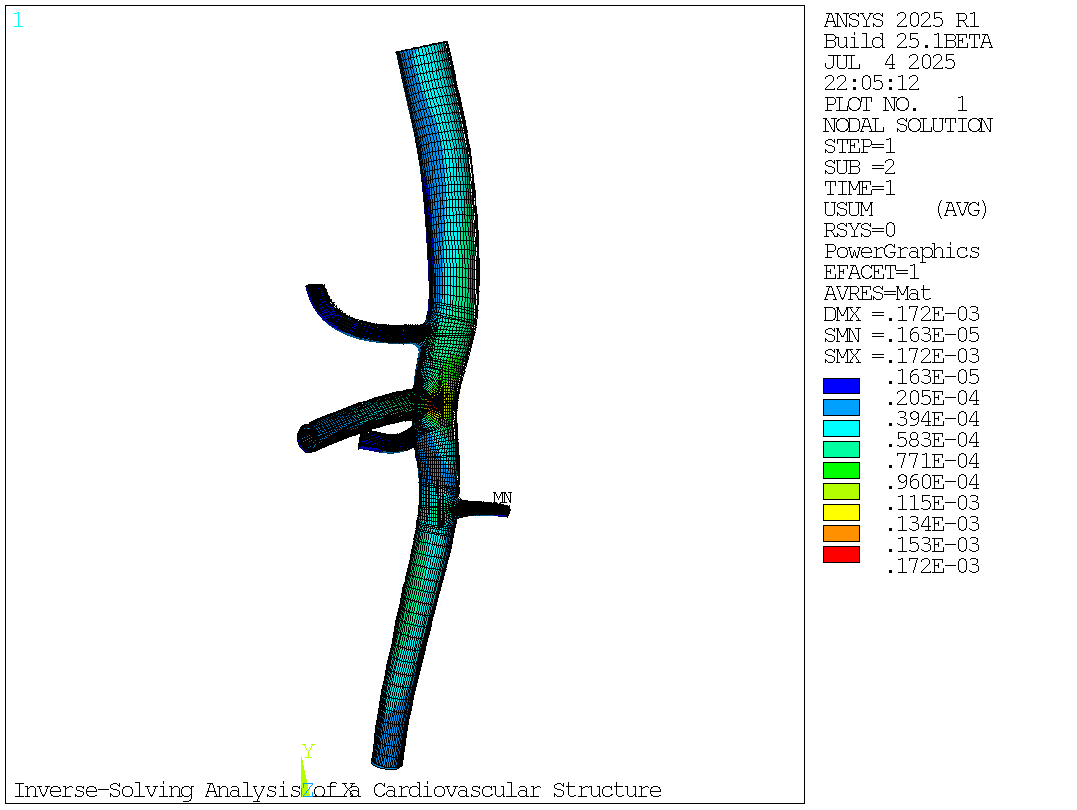
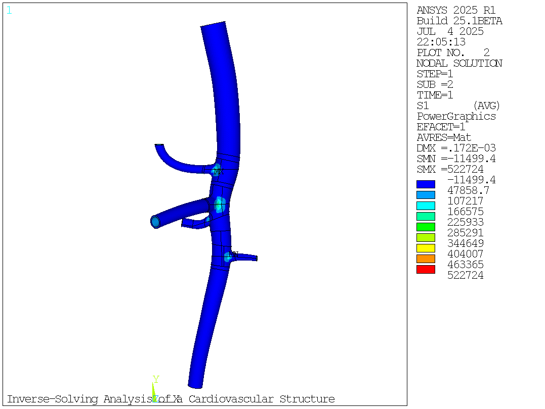
The deformed shape of the abdominal aorta model after the first load step is the zero-pressure geometry:
# Defines the data set to be read from the results file.
mapdl.set(lstep = '1')
mapdl.show("png","rev")

# Total Deformation (USUM) After Inverse Solving (First Load Step)
mapdl.plnsol("u", "sum", 1, 1)
mapdl.get("max_usum_first_loadstep", "plnsol", 0, "max")
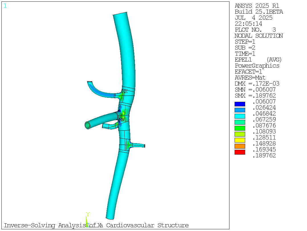
In addition to the zero-pressure geometry, the inverse-solving load step also gives the stress/strain results of the input geometry at end-diastolic pressure (80 mm Hg):
# Maximum Principal Stress After Inverse Solving (First Load Step)
mapdl.plnsol("s", 1)
mapdl.get("max_s1_first_loadstep", "plnsol", 0, "max")

# Maximum Principal Strain After Inverse Solving (First Load Step)
mapdl.plnsol("epel", 1)
mapdl.get("max_epel1_first_loadstep", "plnsol", 0, "max")

mapdl.show("close")
4.2. Load step 2 (forward-solving)#
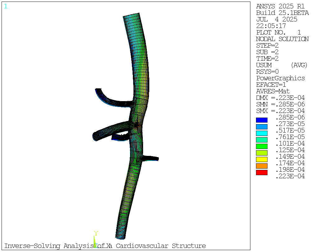
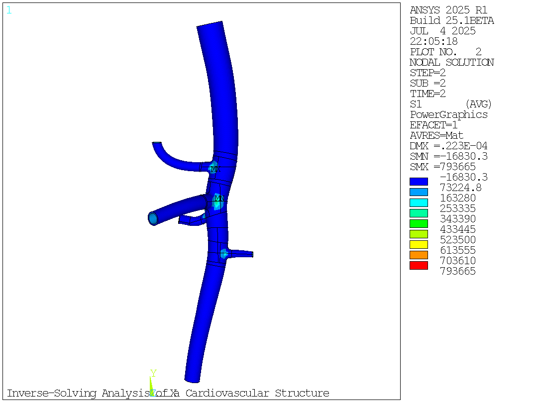
In the second load step, the analysis is continued via forward solving (INVOPT,OFF) and the pressure load is increased until it reaches end-systolic pressure (120 mm Hg):
# Defines the data set to be read from the results file.
mapdl.set(lstep = 'last')
mapdl.show("png","rev")

# Total Deformation (USUM) After Forward Solving (Second Load Step)
mapdl.plnsol("u", "sum", 1, 1)
mapdl.get("max_usum_second_loadstep", "plnsol", 0, "max")

# Maximum Principal Stress After Forward Solving (Second Load Step)
mapdl.plnsol("s", 1)
mapdl.get("max_s1_second_loadstep", "plnsol", 0, "max")

# Maximum Principal Strain Plot of the Abdominal Aorta Model at End-Systolic Pressure (120 mm Hg)
mapdl.plnsol("epel", 1)
mapdl.get("max_epel1_second_loadstep", "plnsol", 0, "max")
mapdl.show("close")

For comparison purposes only, the following figure shows one of the cross-sections in the proximal abdominal aorta at zero-pressure, end-diastolic pressure, and end-systolic pressure conditions:
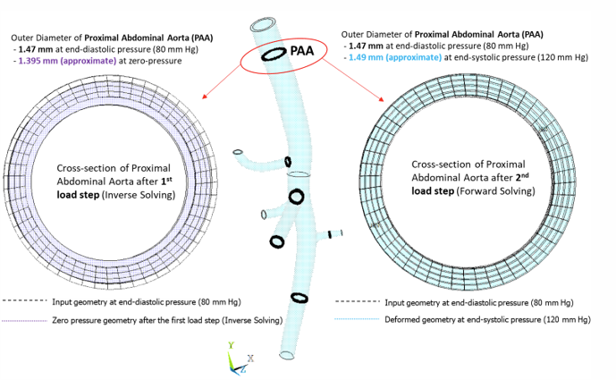
The input geometry is considered at end-diastolic pressure (80 mm Hg), the deformed geometry after the first load step (inverse solving) is at zero-pressure, and the deformed geometry after the second load step is at end-systolic pressure (120 mm Hg). The outer diameters of the cross-section in deformed states are approximately calculated by creating a local cylindrical coordinate system at the approximate center of the deformed cross-section.
When using the inverse-solving method to account for the input geometry at end-diastolic pressure (80 mm Hg) and prestress effects, the actual maximum total deformation is much lower.
5. Exit MAPDL#
mapdl.exit()
6. Recommendations#
When performing a similar type of analysis using inverse-solving, consider the following:
Use a structured mesh with a sufficient number of element layers in the thickness direction.
Doing so captures results more accurately, as a free mesh may give lesser-quality tetrahedral and/or pyramid elements, leading to spurious high-stress concentrations at some locations.
Perform a loop test to verify the results of an inverse-solving analysis.
An inverse-solving analysis followed by a forward-solving analysis, or vice versa, is known as a loop test, as it should always result in the same geometry with the same solution.
Use a reversed sign to apply displacement type loading in the inverse-solving load step.
For more information, see Applying Loads in an inverse-solving Analysis in the Structural Analysis Guide.
7. References#
The following reference works are cited in, or were consulted when creating, this example problem:
Bols, J., Degroote, J., Trachet, B., Verhegghe, B., Segers, P., & Vierendeels, J. (2013). A computational method to assess the in vivo stresses and unloaded configuration of patient-specific blood vessels. Journal of Computational and Applied Mathematics. 246: 10-17.
Trachet, B., Renard, M., DeSantis, G., Staelens, S., DeBacker, J., Antiga, L., Loeys, B., & Segers, P. (2011). An integrated framework to quantitatively link mouse-specific hemodynamics to aneurysm formation in angiotensin II-infused ApoE -/- mice. Annals of Biomedical Engineering. 39: 2430-2444.
Trachet, B., Bols, J., Degroote, J., Verhegghe, B., Stergiopulos, N., Vierendeels, J., & Segers, P. (2015). An animal-specific FSI model of the abdominal aorta in anesthetized mice. Annals of Biomedical Engineering. 43: 1298-1309.
Prendergast, P.J., Lally, C., Daly, S., Reid, A. J., Lee, T. C., Quinn, D., & Dolan, F. (2003). Analysis of prolapse in cardiovascular stents: a constitutive equation for vascular tissue and finite-element modelling. Journal of Biomechanical Engineering. 125(5): 692-699.
8. Input files#
The following files were used in this problem:
Inverse_Analysis_Cardiovascular_Structure.dat – Input file for this example problem.
Comparison_Case.dat – Input file for the comparison case.
For more information, see Obtaining the input files.