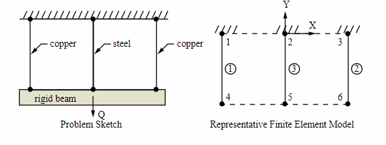
Thermally loaded support structure

Problem description:

• Find the stresses in the copper and steel wire structure shown below. The wires have a cross-sectional area of math:A. The structure is subjected to a load math:Q and a temperature rise of math:Delta T after assembly.

Reference:

• S. Timoshenko, Strength of Materials, Part I, Elementary Theory and Problems, 3rd Edition, D. Van Nostrand Co., Inc., New York, NY, 1955, pg. 30, problem 9.

Analysis type(s):

• Static Analysis ANTYPE=0

Element type(s):

• 3-D Spar (or Truss) Elements (LINK180)

Material properties

• \(E_c = 16 \cdot 10^6 psi\)

• \(E_s = 30 \cdot 10^6 psi\)

• \(\alpha_c = 70 \cdot 10^{-7} in/in-^\circ F\)

• \(\alpha_s = 92 \cdot 10^{-7} in/in-^\circ F\)

Geometric properties:

• \(A = 0.1 in^2\)

Loading:

• \(Q = 4000 lb\)

• \(\Delta T = 10 ^\circ F\)

Analytical equations:

• The compressive force \(X\) is given by the following equation

• \(X = \frac{\Delta T (\alpha_c - \alpha_s) (A_s - E_s) }{1 + \frac{1 E_s A_s}{2 E_c A_c}} + \frac{Q}{1 + \frac{2 E_c A_c}{E_s A_s}}\)

Notes:

• Length of wires (20 in.), spacing between wires (10 in.), and the reference temperature (70°F) are arbitrarily selected. The rigid lower beam is modeled by nodal coupling.

# sphinx_gallery_thumbnail_path = '_static/vm3_setup.png'

from ansys.mapdl.core import launch_mapdl

# start mapdl and clear it
mapdl = launch_mapdl()
mapdl.clear()  # optional as MAPDL just started

# enter verification example mode and the pre-processing routine
mapdl.verify()
mapdl.prep7()

*****MAPDL VERIFICATION RUN ONLY*****
     DO NOT USE RESULTS FOR PRODUCTION

          ***** MAPDL ANALYSIS DEFINITION (PREP7) *****

Define material

Set up the materials and their properties. We are using copper and steel here. - EX - X-direction elastic modulus - ALPX - Secant x - coefficient of thermal expansion

mapdl.antype("STATIC")
mapdl.et(1, "LINK180")
mapdl.sectype(1, "LINK")
mapdl.secdata(0.1)
mapdl.mp("EX", 1, 16e6)
mapdl.mp("ALPX", 1, 92e-7)
mapdl.mp("EX", 2, 30e6)
mapdl.mp("ALPX", 2, 70e-7)
# Define the reference temperature for the thermal strain calculations.
mapdl.tref(70)

REFERENCE TEMPERATURE=  70.000  (TUNIF=  70.000)

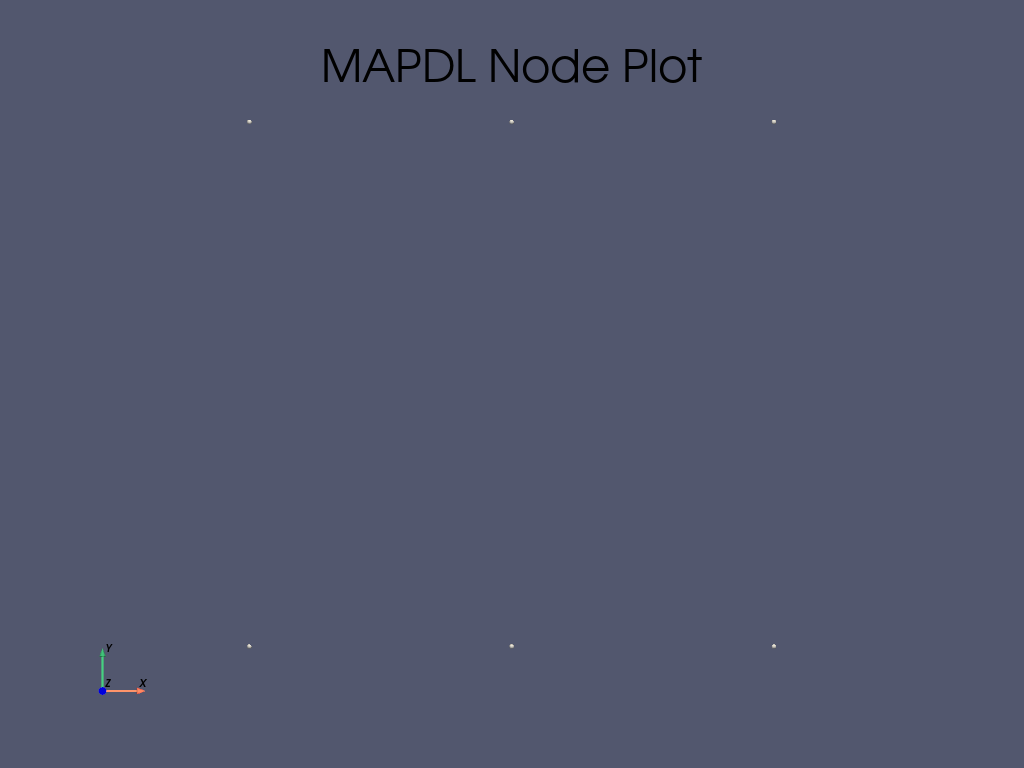
Define geometry: nodes

Set up the nodes and elements. This creates a mesh just like in the problem setup. We create a square of nodes and use fill to add mid-point nodes to two opposite sides.

mapdl.n(1, -10)
mapdl.n(3, 10)
mapdl.fill()
mapdl.n(4, -10, -20)
mapdl.n(6, 10, -20)
mapdl.fill()
mapdl.nplot(nnum=True, cpos="xy")

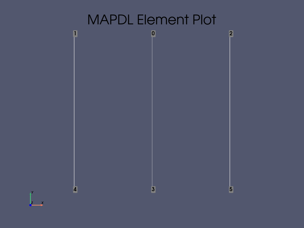
Define geometry: elements

Create two elements (using material #1) that are two sides of our square, as links. Then create a single element using material #2 between the first 2 that is parallel to them.

mapdl.e(1, 4)
mapdl.e(3, 6)
mapdl.mat(2)
mapdl.e(2, 5)
mapdl.eplot(show_node_numbering=True, cpos="xy")

Define boundary conditions

• Couple the degrees of freedom in y-displacement across nodes 5, 4, and 6.

• Fix nodes 1, 2, and 3 in place.

• Apply a force of -4000 in the y-direction to node 5

• Apply a uniform temperature of 80 to the whole body

• Finally, exit the post-processor.

mapdl.cp(1, "UY", 5, 4, 6)
mapdl.d(1, "ALL", "", "", 3)
mapdl.f(5, "FY", -4000)
mapdl.bfunif("TEMP", 80)
mapdl.finish()

***** ROUTINE COMPLETED *****  CP =         0.000

Solve

• Enter solution mode

• Specify a timestep of 1 to be used for this load step

• Solve the system.

mapdl.run("/SOLU")
mapdl.nsubst(1)
mapdl.solve()

*****  MAPDL SOLVE    COMMAND  *****

 *** NOTE ***                            CP =       0.000   TIME= 00:00:00
 There is no title defined for this analysis.
   *****MAPDL VERIFICATION RUN ONLY*****
     DO NOT USE RESULTS FOR PRODUCTION

                       S O L U T I O N   O P T I O N S

   PROBLEM DIMENSIONALITY. . . . . . . . . . . . .3-D
   DEGREES OF FREEDOM. . . . . . UX   UY   UZ
   ANALYSIS TYPE . . . . . . . . . . . . . . . . .STATIC (STEADY-STATE)
   GLOBALLY ASSEMBLED MATRIX . . . . . . . . . . .SYMMETRIC

 *** NOTE ***                            CP =       0.000   TIME= 00:00:00
 Present time 0 is less than or equal to the previous time.  Time will
 default to 1.

 *** NOTE ***                            CP =       0.000   TIME= 00:00:00
 The conditions for direct assembly have been met.  No .emat or .erot
 files will be produced.

 *** NOTE ***                            CP =       0.000   TIME= 00:00:00
 Only 1 process can be used for the distributed memory parallel solution
 for this model due to the presence of the coupling equations in this
 particular model.  Distributed parallel processing has been
 temporarily disabled.

                      L O A D   S T E P   O P T I O N S

   LOAD STEP NUMBER. . . . . . . . . . . . . . . .     1
   TIME AT END OF THE LOAD STEP. . . . . . . . . .  1.0000
   NUMBER OF SUBSTEPS. . . . . . . . . . . . . . .     1
   STEP CHANGE BOUNDARY CONDITIONS . . . . . . . .    NO
   PRINT OUTPUT CONTROLS . . . . . . . . . . . . .NO PRINTOUT
   DATABASE OUTPUT CONTROLS. . . . . . . . . . . .ALL DATA WRITTEN
                                                  FOR THE LAST SUBSTEP



 Range of element maximum matrix coefficients in global coordinates
 Maximum = 150000 at element 0.
 Minimum = 80000 at element 0.

   *** ELEMENT MATRIX FORMULATION TIMES
     TYPE    NUMBER   ENAME      TOTAL CP  AVE CP

        1         3  LINK180       0.000   0.000000
 Time at end of element matrix formulation CP = 0.

 SPARSE MATRIX DIRECT SOLVER.
  Number of equations =           1,    Maximum wavefront =      0
  Memory available (MB) =    0.0    ,  Memory required (MB) =    0.0

 Sparse solver maximum pivot= 0 at node 0 .
 Sparse solver minimum pivot= 0 at node 0 .
 Sparse solver minimum pivot in absolute value= 0 at node 0 .

   *** ELEMENT RESULT CALCULATION TIMES
     TYPE    NUMBER   ENAME      TOTAL CP  AVE CP

        1         3  LINK180       0.000   0.000000

   *** NODAL LOAD CALCULATION TIMES
     TYPE    NUMBER   ENAME      TOTAL CP  AVE CP

        1         3  LINK180       0.000   0.000000
 *** LOAD STEP     1   SUBSTEP     1  COMPLETED.    CUM ITER =      1
 *** TIME =   1.00000         TIME INC =   1.00000      NEW TRIANG MATRIX

Post-processing

• Access the queries functions

• Find a steel node and a copper node

• Then use these to get the steel and copper elements

• Finally extract the stress experienced by each element

mapdl.post1()
q = mapdl.queries
steel_n = q.node(0, 0, 0)
copper_n = q.node(10, 0, 0)
steel_e = q.enearn(steel_n)
copper_e = q.enearn(copper_n)
mapdl.etable("STRS_ST", "LS", 1)
mapdl.etable("STRS_CO", "LS", 1)

stress_steel = mapdl.get("_", "ELEM", steel_e, "ETAB", "STRS_ST")
stress_copper = mapdl.get("_", "ELEM", copper_e, "ETAB", "STRS_CO")

Check results

Now that we have the response we can compare the values to the expected stresses of 19695 and 10152 respectively.

steel_target = 19695
steel_ratio = stress_steel / steel_target
copper_target = 10152
copper_ratio = stress_copper / copper_target

message = f"""
------------------- VM3 RESULTS COMPARISON ---------------------

             |   TARGET   |   Mechanical APDL   |   RATIO
----------------------------------------------------------------
    Steel        {steel_target}        {stress_steel}            {steel_ratio:.6f}
    Copper       {copper_target}        {stress_copper}            {copper_ratio:.6f}

----------------------------------------------------------------

"""
print(message)

------------------- VM3 RESULTS COMPARISON ---------------------

             |   TARGET   |   Mechanical APDL   |   RATIO
----------------------------------------------------------------
    Steel        19695        19695.4844            1.000025
    Copper       10152        10152.2578            1.000025

----------------------------------------------------------------

Stop MAPDL.

mapdl.exit()