Laterally Loaded Tapered Support Structure

Problem description:

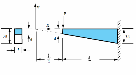
• A cantilever beam of thickness \(t\) and length \(l\) has a depth which tapers uniformly from \(d\) at the tip to \(3d\) at the wall. It is loaded by a force \(F\) at the tip, as shown. Find the maximum bending stress at the mid-length (\(X = l\)) and the fixed end of the beam.

Reference:

• S. H. Crandall, N. C. Dahl, An Introduction to the Mechanics of Solids, McGraw-Hill Book Co., Inc., New York, NY, 1959, pg. 342, problem 7.18.

Analysis type(s):

• Static Analysis ANTYPE=0

Element type(s):

• 2-D 4-Node Sructural Solid Elements (PLANE182)

• 2-D 8-Node Structural Solid Elements (PLANE183)

Material properties

• \(E = 30 \cdot 10^6 psi\)

• \(\nu = 0.0\)

• \(d = 3in\)

• \(t = 2in\)

Geometric properties:

• \(l = 50 in\)

• \(d = 3 in\)

• \(t = 2 in\)

Loading:

• \(F = 4000 lb\)

Notes:

• Two different solutions are obtained. The first solution uses lower order PLANE182 elements and the second solution uses higher order PLANE82 elements. The 2 inch thickness is incorporated by using the plane stress with thickness option. Poisson’s ratio is set to 0.0 to agree with beam theory.

# sphinx_gallery_thumbnail_path = '_static/vm5_setup.png'

Start MAPDL

from ansys.mapdl.core import launch_mapdl

# start mapdl and clear it
mapdl = launch_mapdl()
mapdl.clear()  # optional as MAPDL just started

# enter verification example mode and the pre-processing routine
mapdl.verify()
mapdl.prep7()

*****MAPDL VERIFICATION RUN ONLY*****
     DO NOT USE RESULTS FOR PRODUCTION

          ***** MAPDL ANALYSIS DEFINITION (PREP7) *****

Define material

Set up the material using PLANE182 with a thickness of 2 (using real constants), and create a material with a Young’s modulus of 30e6, and a poisson’s ratio of 0.0 to agree with beam theory.

mapdl.antype("STATIC")
mapdl.et(1, "PLANE182", kop1=2, kop3=3)
mapdl.r(1, 2)
mapdl.mp("EX", 1, 30e6)
mapdl.mp("NUXY", 1, 0.0)

MATERIAL          1     NUXY =   0.000000

Define geometry

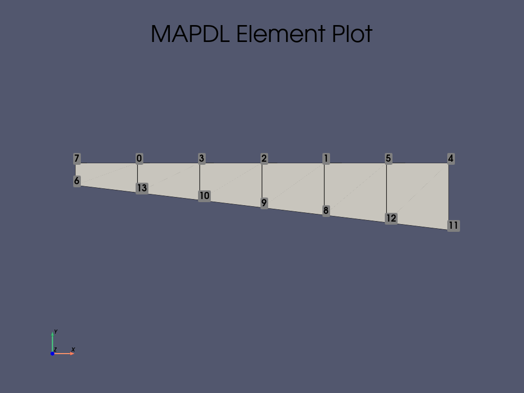
Set up the nodes and elements. This creates a mesh just like in the problem setup.

mapdl.n(1, 25)
mapdl.n(7, 75)
mapdl.fill()
mapdl.n(8, 25, -3)
mapdl.n(14, 75, -9)
mapdl.fill()
mapdl.e(2, 1, 8, 9)
mapdl.egen(6, 1, 1)
mapdl.eplot(show_node_numbering=True, cpos="xy")

Define boundary conditions

Fix the nodes at the larger end (the “wall” end) and apply a vertical force to the whole structure.

# constrain nodes at fixed end
mapdl.nsel("S", "LOC", "X", 75)
mapdl.d("ALL", "ALL")
mapdl.nsel("ALL")
mapdl.f(1, "FY", -4000)
mapdl.finish()

***** ROUTINE COMPLETED *****  CP =         0.000

Solve

Enter solution mode and solve the system.

mapdl.run("/SOLU")
mapdl.solve()
mapdl.finish()

FINISH SOLUTION PROCESSING


 ***** ROUTINE COMPLETED *****  CP =         0.000

Post-processing

Enter post-processing. Get the stress at the fixed end and the mid point of the structure by querying the stress at nodes closest to these locations. We’ve gathered the code into a function because we’ll have use for it later.

def fetch_mid_and_end_stress(m):
    q = m.queries
    m.post1()
    end = q.node(75.0, 0.0, 0.0)
    fixed_end_stress = m.get_value("NODE", end, "S", "X")
    mid = q.node(50.0, 0.0, 0.0)
    mid_stress = m.get_value("NODE", mid, "S", "EQV")
    return fixed_end_stress, mid_stress


fixed_end_stress_182, mid_stress_182 = fetch_mid_and_end_stress(mapdl)

Plotting

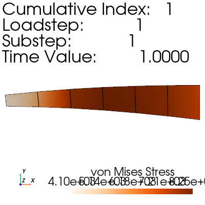
View the equivalent stress, and displacement, of the cantilever with a displacement_factor of 26 to scale up the deformation to a visible amount.

result = mapdl.result
result.plot_principal_nodal_stress(
    0,
    "SEQV",
    show_edges=True,
    show_displacement=True,
    displacement_factor=26.0,
    cmap="Oranges",
    cpos="xy",
)

Redo with Plane 183

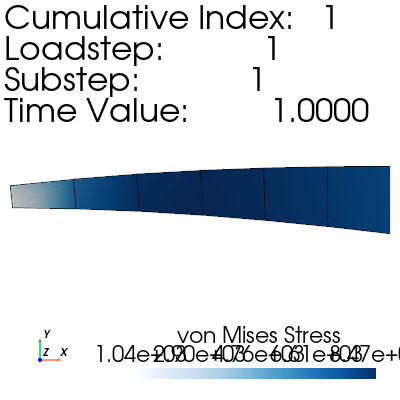
Now we need to perform the simulation again but this time using the PLANE183 element type. We additionally remove midside nodes with emid.

mapdl.prep7()
mapdl.et(1, "PLANE183", kop3=3)
mapdl.emid()
mapdl.nsel("R", "LOC", "X", 75)
mapdl.nsel("R", "LOC", "Y", -4.5)

mapdl.d("ALL", "ALL")
mapdl.nsel("ALL")
mapdl.finish()
mapdl.run("/SOLU")
mapdl.solve()
mapdl.finish()

mapdl.post1()
# reuse our function from earlier
fixed_end_stress_183, mid_stress_183 = fetch_mid_and_end_stress(mapdl)
mapdl.finish()

result = mapdl.result
result.plot_principal_nodal_stress(
    0,
    "SEQV",
    show_edges=True,
    show_displacement=True,
    displacement_factor=26.0,
    cmap="Blues",
    cpos="xy",
)

Check results

Now that we have the stresses we can compare them to the expected values of stress at the midpoint (8333) and the fixed end (7407) for both simulations.

results_182 = f"""
-----------------  PLANE 182 RESULTS COMPARISON  ----------------
|    LABEL    |   TARGET   |   Mechanical APDL   |   RATIO
   mid stress      8333        {mid_stress_182:.2f}               {mid_stress_182 / 8333:.2f}
   end stress      7407        {fixed_end_stress_182:.2f}         {fixed_end_stress_182 / 7407:.2f}
----------------------------------------------------------------
"""

results_183 = f"""
-----------------  PLANE 183 RESULTS COMPARISON  ----------------
|    LABEL    |   TARGET   |   Mechanical APDL   |   RATIO
   mid stress      8333        {mid_stress_183:.2f}               {mid_stress_183 / 8333:.2f}
   end stress      7407        {fixed_end_stress_183:.2f}         {fixed_end_stress_183 / 7407:.2f}
----------------------------------------------------------------
"""
print(results_182)
print(results_183)

-----------------  PLANE 182 RESULTS COMPARISON  ----------------
|    LABEL    |   TARGET   |   Mechanical APDL   |   RATIO
   mid stress      8333        8163.66               0.98
   end stress      7407        7151.10         0.97
----------------------------------------------------------------


-----------------  PLANE 183 RESULTS COMPARISON  ----------------
|    LABEL    |   TARGET   |   Mechanical APDL   |   RATIO
   mid stress      8333        8363.71               1.00
   end stress      7407        7408.98         1.00
----------------------------------------------------------------

Stop MAPDL.

mapdl.exit()