Note
Go to the end to download the full example code.
Plastic compression of a pipe assembly#
- Problem description:
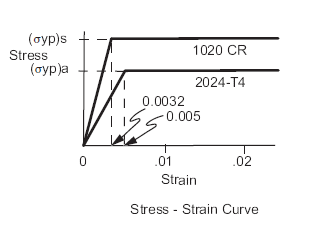
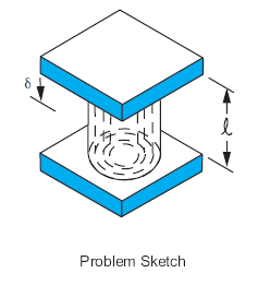
Two coaxial tubes, the inner one of 1020 CR steel and cross-sectional area \(A_{\mathrm{s}}\), and the outer one of 2024-T4 aluminum alloy and of area \(A_{\mathrm{a}}\), are compressed between heavy, flat end plates, as shown below. Determine the load-deflection curve of the assembly as it is compressed into the plastic region by an axial displacement. Assume that the end plates are so stiff that both tubes are shortened by exactly the same amount.
- Reference:
S. H. Crandall, N. C. Dahl, An Introduction to the Mechanics of Solids, McGraw-Hill Book Co., Inc., New York, NY, 1959, pg. 180, ex. 5.1.
- Analysis type(s):
Static, Plastic Analysis (
ANTYPE=0)
- Element type(s):
Plastic Straight Pipe Element (PIPE288)
4-node finite strain shell (SHELL181)
3d structural solid elements (SOLID185)

- Material properties
\(E_{\mathrm{s}} = 26875000\,psi\)
\(\sigma_{\mathrm{(yp)s}} = 86000\,psi\)
\(E_{\mathrm{a}} = 11000000\,psi\)
\(\sigma_{\mathrm{(yp)a}} = 55000\,psi\)
\(\nu = 0.3\)
- Geometric properties:
\(l = 10\,in\)
\(A_{\mathrm{s}} = 7\,in^2\)
\(A_{\mathrm{a}} = 12\,in^2\)
- Loading:
1st load step: \(\delta = 0.032\,in\)
2nd load step: \(\delta = 0.050\,in\)
3rd load step: \(\delta = 0.100\,in\)
- Analysis assumptions and modeling notes:
The following tube dimensions, which provide the desired cross-sectional areas, are arbitrarily chosen:
Inner (steel) tube: inside radius = 1.9781692 in., wall thickness = 0.5 in.
Outer (aluminum) tube: inside radius = 3.5697185 in., wall thickness = 0.5 in.
The problem can be solved in three ways:
using
PIPE288- the plastic straight pipe elementusing
SOLID185- the 3d structural solid elementusing
SHELL181- the 4-node finite strain shell
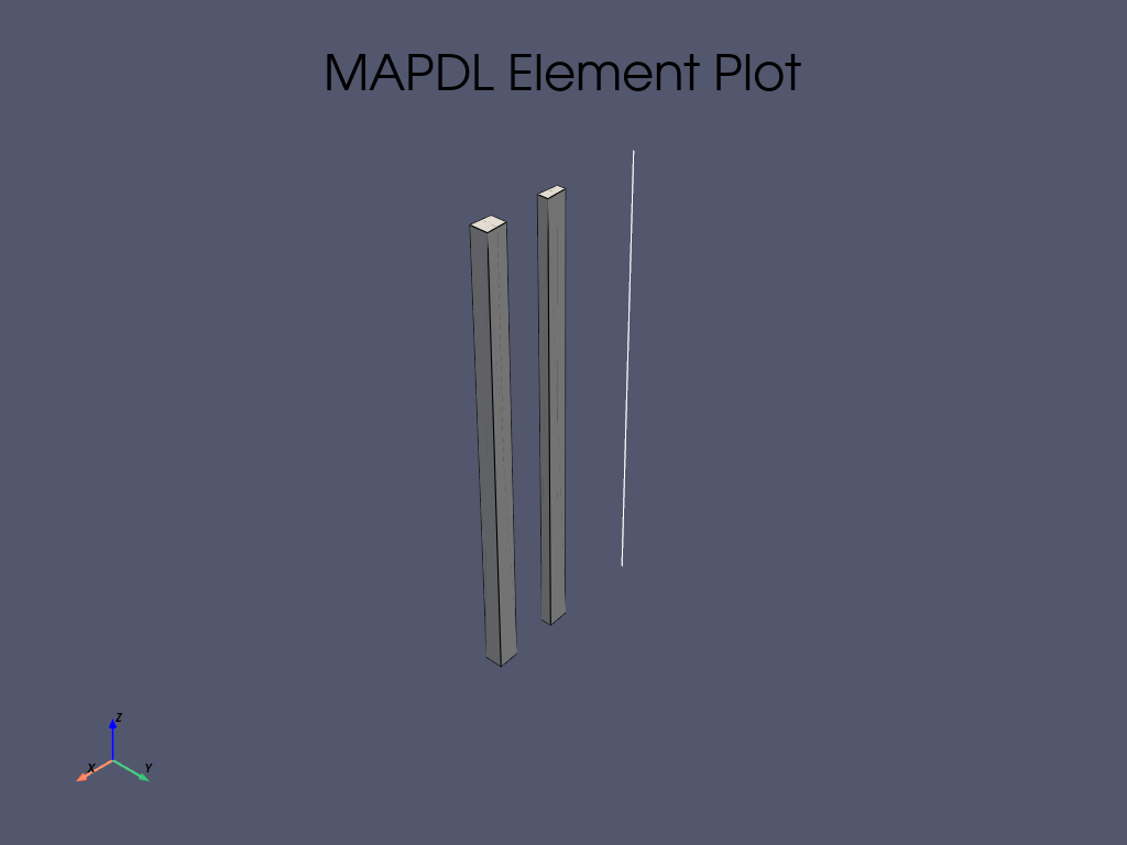
In the SOLID185 and SHELL181 cases, since the problem is axisymmetric, only a one element \(\theta\) -sector is modeled. A small angle \(\theta = 6°\) is arbitrarily chosen to reasonably approximate the circular boundary with straight sided elements. The nodes at the boundaries have the
UX(radial) degree of freedom coupled. In the SHELL181 model, the nodes at the boundaries additionally have theROTYdegree of freedom coupled.
# sphinx_gallery_thumbnail_path = '_static/vm7_setup.png'
Start MAPDL#
Start MAPDL and import Numpy and Pandas libraries.
from ansys.mapdl.core import launch_mapdl
import matplotlib.pyplot as plt
import numpy as np
import pandas as pd

# Start MAPDL.
mapdl = launch_mapdl()
Pre-processing#
Enter verification example mode and the pre-processing routine.
mapdl.clear()
mapdl.verify()
mapdl.prep7(mute=True)
Parameterization#
Define element type#
Set up the element types .
# Element type PIPE288.
mapdl.et(1, "PIPE288")

# Special features are defined by keyoptions of pipe element.
# KEYOPT(4)(2)
# Hoop strain treatment:
# Thick pipe theory.
mapdl.keyopt(1, 4, 2)  # Cubic shape function

# Element type SOLID185.
mapdl.et(2, "SOLID185")

# Element type SHELL181.
mapdl.et(3, "SHELL181")  # FULL INTEGRATION

# Special features are defined by keyoptions of shell element.
# KEYOPT(3)(2)
# Integration option:
# Full integration with incompatible modes.
mapdl.keyopt(3, 3, 2)

# Print
print(mapdl.etlist())
LIST ELEMENT TYPES FROM        1 TO        3 BY        1
   *****MAPDL VERIFICATION RUN ONLY*****
     DO NOT USE RESULTS FOR PRODUCTION

 ELEMENT TYPE        1 IS PIPE288      3-D 2-NODE PIPE
  KEYOPT( 1- 6)=        0      0      0        2      0      0
  KEYOPT( 7-12)=        0      0      0        0      0      0
  KEYOPT(13-18)=        0      0      0        0      0      0

 ELEMENT TYPE        2 IS SOLID185     3-D 8-NODE STRUCTURAL SOLID
  KEYOPT( 1- 6)=        0      0      0        0      0      0
  KEYOPT( 7-12)=        0      0      0        0      0      0
  KEYOPT(13-18)=        0      0      0        0      0      0

 ELEMENT TYPE        3 IS SHELL181     4-NODE SHELL
  KEYOPT( 1- 6)=        0      0      2        0      0      0
  KEYOPT( 7-12)=        0      0      0        0      0      0
  KEYOPT(13-18)=        0      0      0        0      0      0

 CURRENT NODAL DOF SET IS  UX    UY    UZ    ROTX  ROTY  ROTZ
  THREE-DIMENSIONAL MODEL
Define material#
Set up the material properties.
Young modulus of steel is: \(E_{\mathrm{s}} = 26875000\,psi\),
Yield strength of steel is: \(\sigma_{\mathrm{(yp)s}} = 86000\, psi\),
Young modulus of aluminum is: \(E_{\mathrm{a}} = 11000000\,psi\),
Yield strength of aluminum is: \(\sigma_{\mathrm{(yp)a}} = 55000\,psi\),
Poisson’s ratio is: \(\nu = 0.3\)
# Steel material model
# Define Young's moulus and Poisson ratio for steel.
mapdl.mp("EX", 1, 26.875e6)
mapdl.mp("PRXY", 1, 0.3)

# Define non-linear material properties for steel.
mapdl.tb("BKIN", 1, 1)
mapdl.tbtemp(0)
mapdl.tbdata(1, 86000, 0)

# Aluminum material model
# Define Young's moulus and Poisson ratio for aluminum.
mapdl.mp("EX", 2, 11e6)
mapdl.mp("PRXY", 2, 0.3)

# Define non-linear material properties for aluminum.
mapdl.tb("BKIN", 2, 1)
mapdl.tbtemp(0)
mapdl.tbdata(1, 55000, 0)

# Print
print(mapdl.mplist())
LIST MATERIALS        1 TO        2 BY        1
  PROPERTY= ALL

 MATERIAL NUMBER        1

      TEMP        EX
               0.2687500E+08

      TEMP        PRXY
               0.3000000

 MATERIAL NUMBER        2

      TEMP        EX
               0.1100000E+08

      TEMP        PRXY
               0.3000000
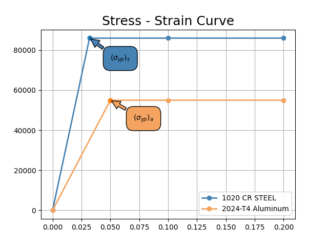
Plot stress - strain curve#
Use Matplotlib library to plot material model curves of steel and aluminum.
# Define stress - strain properties of the steel.
steel = {"stress_s": [0, 86000, 86000, 86000], "strain_s": [0, 0.032, 0.1, 0.2]}

# Define yielding strength point of the steel on the curve.
xp = steel["strain_s"][1]
yp = steel["stress_s"][1]

# Set up the settings of the steel curve.
plt.plot(
    steel["strain_s"],
    steel["stress_s"],
    label="1020 CR STEEL",
    linewidth=2,
    color="steelblue",
    linestyle="-",
    marker="o",
)
plt.plot(xp, yp, marker="o")

# Annotation settings
plt.annotate(
    r"${(\sigma_{yp})_s}$",
    xy=(xp, yp),
    xytext=(0.05, 75000),
    arrowprops=dict(facecolor="steelblue", shrink=0.05),
    bbox=dict(facecolor="steelblue", edgecolor="black", boxstyle="round, pad=1"),
)

# Define stress - strain properties of the aluminum.
aluminum = {"stress_a": [0, 55000, 55000, 55000], "strain_a": [0, 0.05, 0.1, 0.2]}

# Define yielding strength point of the aluminum on the curve.
xp = aluminum["strain_a"][1]
yp = aluminum["stress_a"][1]

# Set up the settings of the aluminum curve.
plt.plot(
    aluminum["strain_a"],
    aluminum["stress_a"],
    label="2024-T4 Aluminum",
    linewidth=2,
    color="sandybrown",
    linestyle="-",
    marker="o",
)
plt.plot(xp, yp, marker="o")

# Annotation settings
plt.annotate(
    r"${(\sigma_{yp})_a}$",
    xy=(xp, yp),
    xytext=(0.07, 45000),
    arrowprops=dict(facecolor="sandybrown", shrink=0.05),
    bbox=dict(facecolor="sandybrown", edgecolor="black", boxstyle="round, pad=1"),
)

plt.grid(True)
plt.legend()
plt.title("Stress - Strain Curve", fontsize=18)
plt.show()
Define section#
Set up the cross-section properties for a shell and pipe elements.
# Shell cross-section for inside tube(steel).
mapdl.sectype(1, "SHELL")

# Thickness (SHELL181)
mapdl.secdata(0.5, 1, 0, 5)

# Shell cross-section for outside tube(aluminum).
mapdl.sectype(2, "SHELL")

# Thickness (SHELL181)
mapdl.secdata(0.5, 2, 0, 5)

# Define pipe cross-section for inside tube(steel).
mapdl.sectype(3, "PIPE")

# Outside diameter and wall thickness settings for inside tube(PIPE288).
mapdl.secdata(4.9563384, 0.5)

# Pipe cross-section for outside tube(aluminum) .
mapdl.sectype(4, "PIPE")

# Outside diameter and wall thickness settings for outside tube (PIPE288).
mapdl.secdata(8.139437, 0.5)

# Print the section properties for all sections.
print(mapdl.slist())
*****MAPDL VERIFICATION RUN ONLY*****
     DO NOT USE RESULTS FOR PRODUCTION

 LIST SECTION ID SETS         1 TO         4 BY        1

   SECTION ID NUMBER:             1
   SHELL SECTION TYPE:
   SHELL SECTION NAME IS:
   SHELL SECTION DATA SUMMARY:
    Number of Layers    =      1
    Total Thickness     =     0.500000

  Layer      Thickness   MatID   Ori. Angle  Num Intg. Pts

      1        0.5000         1        0.0000     5

    Shell Section is offset to MID surface of Shell

    Section Solution Controls
    User Transverse Shear Stiffness (11)=  0.0000
                                    (22)=  0.0000
                                    (12)=  0.0000
    Added Mass Per Unit Area            =  0.0000
    Hourglass Scale Factor; Membrane    =  1.0000
                            Bending     =  1.0000
    Drill Stiffness Scale Factor        =  1.0000
    Bending Stiffness Scale Factor      =  1.0000

   SECTION ID NUMBER:             2
   SHELL SECTION TYPE:
   SHELL SECTION NAME IS:
   SHELL SECTION DATA SUMMARY:
    Number of Layers    =      1
    Total Thickness     =     0.500000

  Layer      Thickness   MatID   Ori. Angle  Num Intg. Pts

      1        0.5000         2        0.0000     5

    Shell Section is offset to MID surface of Shell

    Section Solution Controls
    User Transverse Shear Stiffness (11)=  0.0000
                                    (22)=  0.0000
                                    (12)=  0.0000
    Added Mass Per Unit Area            =  0.0000
    Hourglass Scale Factor; Membrane    =  1.0000
                            Bending     =  1.0000
    Drill Stiffness Scale Factor        =  1.0000
    Bending Stiffness Scale Factor      =  1.0000

   SECTION ID NUMBER:           3
   PIPE SECTION NAME IS:
   PIPE SECTION DATA SUMMARY:
    Outside Diameter     =  4.9563
    Thickness            = 0.50000
    Area                 =  6.9946
    Iyy                  =  17.559
    Torsion Constant     =  35.118
    Shear Correction-yy  = 0.50995

   SECTION ID NUMBER:           4
   PIPE SECTION NAME IS:
   PIPE SECTION DATA SUMMARY:
    Outside Diameter     =  8.1394
    Thickness            = 0.50000
    Area                 =  11.991
    Iyy                  =  87.735
    Torsion Constant     =  175.47
    Shear Correction-yy  = 0.50305
Define geometry#
Set up the nodes and create the elements through the nodes.
# Generate nodes and elements for PIPE288.
mapdl.n(1, x=0, y=0, z=0)
mapdl.n(2, x=0, y=0, z=10)

# Create element for steel(inside) tube cross-section.
mapdl.mat(1)
mapdl.secnum(3)
mapdl.e(1, 2)

# Create element for aluminum(outside) tube cross-section.
mapdl.mat(2)
mapdl.secnum(4)
mapdl.e(1, 2)

# Activate the global cylindrical coordinate system.
mapdl.csys(1)

# Generate nodes and elements for SOLID185.
mapdl.n(node=101, x=1.9781692)
mapdl.n(node=101, x=1.9781692)
mapdl.n(node=102, x=2.4781692)
mapdl.n(node=103, x=3.5697185)
mapdl.n(node=104, x=4.0697185)
mapdl.n(node=105, x=1.9781692, z=10)
mapdl.n(node=106, x=2.4781692, z=10)
mapdl.n(node=107, x=3.5697185, z=10)
mapdl.n(node=108, x=4.0697185, z=10)

# Generate 2nd set of nodes to form a theta degree slice.
mapdl.ngen(itime=2, inc=10, node1=101, node2=108, dy=theta)

# Rotate nodal coordinate systems into the active system.
mapdl.nrotat(node1=101, node2=118, ninc=1)

# Create elements for the inside (steel) tube.
mapdl.type(2)
mapdl.mat(1)
mapdl.e(101, 102, 112, 111, 105, 106, 116, 115)

# Create elements for the outside (aluminum) tube
mapdl.mat(2)
mapdl.e(103, 104, 114, 113, 107, 108, 118, 117)

# Generate nodes.
mapdl.n(node=201, x=2.2281692)
mapdl.n(node=203, x=2.2281692, z=10)
mapdl.n(node=202, x=3.8197185)
mapdl.n(node=204, x=3.8197185, z=10)

# Generate nodes to form a theta degree slice
mapdl.ngen(itime=2, inc=4, node1=201, node2=204, dy=theta)

# Create element for steel (inside) tube cross-section.
mapdl.type(3)
mapdl.secnum(1)
mapdl.e(203, 201, 205, 207)

# Create element for aluminum (outside) tube cross-section.
mapdl.secnum(2)
mapdl.e(204, 202, 206, 208)

# Plot element model to demonstrate the axisymmetric element model.
cpos = [
    (19.67899462804619, 17.856836088414664, 22.644135378046194),
    (2.03485925, 0.21270071036846988, 5.0),
    (0.0, 0.0, 1.0),
]
mapdl.eplot(cpos=cpos)
[82, 87, 110]
Define boundary conditions#
Application of boundary conditions (BC) for simplified axisymmetric model.
# Apply constraints to the PIPE288 model.
# Fix all DOFs for bottom end of PIPE288.
mapdl.d(node=1, lab="ALL")

# Allow only UZ DOF at top end of the PIPE288.
mapdl.d(node=2, lab="UX", lab2="UY", lab3="ROTX", lab4="ROTY", lab5="ROTZ")

# Apply constraints to SOLID185 and SHELL181 models"
# Couple nodes at boundary in radial direction for SOLID185.
mapdl.cp(nset=1, lab="UX", node1=101, node2=111, node3=105, node4=115)
mapdl.cpsgen(itime=4, nset1=1)

# Couple nodes at boundary in radial direction for the SHELL181.
mapdl.cp(5, lab="UX", node1=201, node2=205, node3=203, node4=20)
mapdl.cpsgen(itime=2, nset1=5)

# Couple nodes at boundary in ROTY direction for SHELL181.
mapdl.cp(7, lab="ROTY", node1=201, node2=205)
mapdl.cpsgen(itime=4, nset1=7)

# Select only nodes in SOLID185 and SHELL181 models.
mapdl.nsel(type_="S", item="NODE", vmin=101, vmax=212)

# Select only nodes at theta = 0 from the selected set.
mapdl.nsel("R", "LOC", "Y", 0)

# Apply symmetry boundary conditions.
mapdl.dsym("SYMM", "Y", 1)

# Select only nodes in SOLID185 and SHELL181 models.
mapdl.nsel(type_="S", item="NODE", vmin=101, vmax=212)

# elect nodes at theta from the selected set.
mapdl.nsel("R", "LOC", "Y", theta)

# Apply symmetry boundary conditions.
mapdl.dsym("SYMM", "Y", 1)

# Select all nodes and reselect only nodes at Z = 0.
mapdl.nsel("ALL")
mapdl.nsel("R", "LOC", "Z", 0)

# Constrain bottom nodes in Z direction.
mapdl.d("ALL", "UZ", 0)

# Select all nodes.
mapdl.nsel("ALL")
mapdl.finish(mute=True)
Solve#
Enter solution mode and solve the system.
# Start solution procedure.
mapdl.slashsolu()

# Define solution function.
def solution(deflect):
    mapdl.nsel("R", "LOC", "Z", 10)
    mapdl.d(node="ALL", lab="UZ", value=deflect)
    mapdl.nsel("ALL")
    mapdl.solve()


# Run each load step to reproduce needed deflection subsequently.
# Load step 1
solution(deflect=defl_ls1)

# Load step 2
solution(deflect=defl_ls2)

# Load step 3
solution(deflect=defl_ls3)
mapdl.finish(mute=True)
Post-processing#
Enter post-processing.
# Enter the post-processing routine.
mapdl.post1(mute=True)
Getting loads#
Set up the function to get load values of each load step of the simplified axisymmetric model and convert it to the full model.
def getload():

    # Select the nodes in the PIPE288 element model.
    mapdl.nsel(type_="S", item="NODE", vmin=1, vmax=2)
    mapdl.nsel("R", "LOC", "Z", 0)

    # Sum the nodal force contributions of elements.
    mapdl.fsum()

    # Extrapolation of the force results in the full 360 (deg) model.
    load_288 = mapdl.get_value("FSUM", 0, "ITEM", "FZ")

    # Select the nodes in the SOLID185 element model.
    mapdl.nsel(type_="S", item="NODE", vmin=101, vmax=118)
    mapdl.nsel("R", "LOC", "Z", 0)
    mapdl.fsum()

    # Get the force value of the simplified model.
    load_185_theta = mapdl.get_value("FSUM", 0, "ITEM", "FZ")

    # Extrapolation of the force results in the full 360 (deg) model.
    load_185 = load_185_theta * 360 / theta

    # Select the nodes in the SHELL181 element model.
    mapdl.nsel("S", "NODE", "", 201, 212)
    mapdl.nsel("R", "LOC", "Z", 0)

    # Sum the nodal force contributions of elements.
    mapdl.fsum()

    # Get the force value of the simplified model.
    load_181_theta = mapdl.get_value("FSUM", 0, "ITEM", "FZ")

    # Extrapolation of the force results in the full 360 (deg) model.
    load_181 = load_181_theta * 360 / theta

    # Return load results of each element model.
    return abs(round(load_288, 0)), abs(round(load_185, 0)), abs(round(load_181, 0))
Getting loads for each load step#
Obtain the loads of the model using getload() function.
# Activate load step 1 and extract load data.
mapdl.set(1, 1)
pipe288_ls1, solid185_ls1, shell181_ls1 = getload()

# Activate load step 2 and extract load data.
mapdl.set(2, 1)
pipe288_ls2, solid185_ls2, shell181_ls2 = getload()

# Activate load step 3 and extract load data.
mapdl.set(3, 1)
pipe288_ls3, solid185_ls3, shell181_ls3 = getload()
Check results#
Finally we have the results of the loads for the simplified axisymmetric model,
which can be compared with expected target values for models with PIPE288,
SOLID185, and SHELL181 elements. Loads expected for each load step are:
1st load step with deflection \(\delta = 0.032 (in)\) has \(load_1 = 1024400\,(lb)\).
2nd load step with deflection \(\delta = 0.05 (in)\) has \(load_2 = 1262000\,(lb)\).
3rd load step with deflection \(\delta = 0.1 (in)\) has \(load_3 = 1262000\,(lb)\).
target_res = np.asarray(
    [1024400, 1262000, 1262000, 1024400, 1262000, 1262000, 1024400, 1262000, 1262000]
)

simulation_res = np.asarray(
    [
        pipe288_ls1,
        pipe288_ls2,
        pipe288_ls2,
        solid185_ls1,
        solid185_ls2,
        solid185_ls3,
        shell181_ls1,
        shell181_ls2,
        shell181_ls3,
    ]
)

main_columns = {
    "Target": target_res,
    "Mechanical APDL": simulation_res,
    "Ratio": list(np.divide(simulation_res, target_res)),
}

row_tuple = [
    ("PIPE288", "Load, lb for Deflection = 0.032 in"),
    ("PIPE288", "Load, lb for Deflection = 0.05 in"),
    ("PIPE288", "Load, lb for Deflection = 0.1 in"),
    ("SOLID185", "Load, lb for Deflection = 0.032 in"),
    ("SOLID185", "Load, lb for Deflection = 0.05 in"),
    ("SOLID185", "Load, lb for Deflection = 0.1 in"),
    ("SHELL181", "Load, lb for Deflection = 0.032 in"),
    ("SHELL181", "Load, lb for Deflection = 0.05 in"),
    ("SHELL181", "Load, lb for Deflection = 0.1 in"),
]

index_names = ["Element Type", "Load Step"]
row_indexing = pd.MultiIndex.from_tuples(row_tuple)
df = pd.DataFrame(main_columns, index=row_indexing)

df.style.set_caption("Results Comparison",).set_table_styles(
    [
        {
            "selector": "th.col_heading",
            "props": [
                ("background-color", "#FFEFD5"),
                ("color", "black"),
                ("border", "0.5px solid black"),
                ("font-style", "italic"),
                ("text-align", "center"),
            ],
        },
        {
            "selector": "th.row_heading",
            "props": [
                ("background-color", "#FFEFD5"),
                ("color", "black"),
                ("border", "0.5px solid black"),
                ("font-style", "italic"),
                ("text-align", "center"),
            ],
        },
        {"selector": "td:hover", "props": [("background-color", "#FFF8DC")]},
        {"selector": "th", "props": [("max-width", "120px")]},
        {"selector": "", "props": [("border", "0.5px solid black")]},
        {
            "selector": "caption",
            "props": [
                ("color", "black"),
                ("font-style", "italic"),
                ("font-size", "24px"),
                ("text-align", "center"),
            ],
        },
    ],
).set_properties(
    **{
        "background-color": "#FFFAFA",
        "color": "black",
        "border-color": "black",
        "border-width": "0.5px",
        "border-style": "solid",
        "text-align": "center",
    }
).format(
    "{:.3f}"
)
Stop MAPDL#
mapdl.exit()
Total running time of the script: (0 minutes 1.604 seconds)