PSD Analysis of 40-Story Building Under Wind Load Excitation

Problem description:

• A 40-story building is modeled using spring-damper (COMBIN14) and point mass elements (MASS21). The stiffness represents the linear elastic massless column and the mass of each floor is concentrated at the floor level, as shown in Figure: Finite Element Representation of 40-Story Building Using Spring-Mass Damper System.

• The wind load excitation is applied at discrete floor levels along the wind motion. Because natural strong winds are turbulent in nature with randomly fluctuating wind velocities, a probabilistic approach like Power Spectral Density (PSD) analysis is the most suitable approach to analyze such structures. This analysis is performed to calculate the response PSD of the 40th floor.

Reference:

• Yang, J.N., Lin, Y.K., “Along-Wind Motion of Multistorey Building”, ASCE Publications, April 1981.

Analysis type(s):

• Modal Analysis ANTYPE=2

• PSD Analysis ANTYPE=8

Element type(s):

• Spring-Damper Element (COMBIN14)

• Structural Point Mass Element (MASS21)

Material properties:

• Floor mass, \(m = 1.29 \times 10^6 kg\)

• Column stiffness, \(K = 1 \cdot 10^9 N/m\)

• Damping coefficient, \(\beta = 2.155 \times 10^4 N/m/sec\)

Geometric properties:

• Number of stories, \(N = 40\)

• Story height, \(h = 4 m\)

Loading (Aerodynamics Properties):

• Wind load tributary area, \(A_w = 192 m^2\)

• Gradient height, \(Z_g = 300 m\)

• Gradient wind velocity, \(U_g = 44.69 m/sec\)

• Reference mean wind velocity at 10 m height, \(U_r = 11.46 m/sec\)

• Drag coefficient, \(C_d = 1.2\)

• Air density, \(\rho = 1.23 kg/m^3\)

• Ground surface drag coefficient, \(K_o = 0.03\)

• Exponent for the mean-wind-profile power law, \(\alpha = 0.4\)

• Constant term, \(C_1 = 7.7\)

Notes:

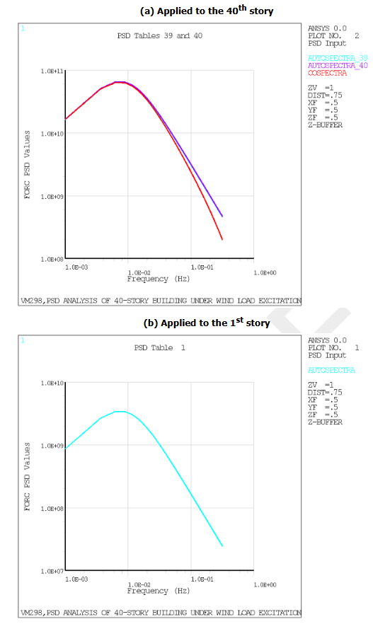
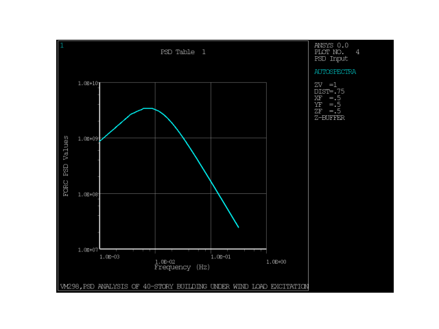
• Partly correlated wind excitation PSD spectrum (Davenport spectrum) is applied at each floor. For illustration, see Figure: Partly Correlated Wind Excitation PSD Spectrum (Davenport Spectrum).

Analysis Assumptions and Modeling Notes:

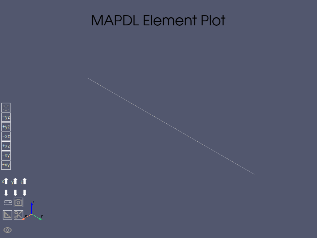
• The 40-story building is modeled using 1-D spring-damper system with one end fixed at its foundation. The motion of the tall building is allowed along the wind direction only.

• The damping in the structure is based on material beta damping using MP,BETD.

• The modal analysis is performed using the Lanczos eigensolver. Only the first frequency is used in the subsequent PSD analysis.

• The PSD analysis loading consists of partly correlated wind excitation PSD applied at each of the floors. The different wind spectrum curves are calculated as APDL array parameters and input with PSDVAL and COVAL. In this example, the displacement response PSD at the top floor is calculated and compared with the reference curve. Using this calculated response PSD, the standard deviation is calculated and compared with the reference value.

Postprocessing:

• Displacement response at the top floor (40th floor) is calculated.

• The response PSD is computed and plotted.

• The standard deviation of the response PSD is calculated.

Reference results:

• Modal frequency of first mode, \(\omega_1 = 1.02 rad/sec\)

• Standard deviation of response PSD at the top floor, \(\sigma_{X40} = 4.65\cdot 10^{-2} m\)

Additional Notes:

• The model uses COMBIN14 elements for spring-damper representation and MASS21 elements for point mass representation.

• The wind load is applied as a power spectral density (PSD) analysis.

• The results are visualized using plots of the response PSD and displacement.

• The model is verified against the reference values provided in the literature.

• The results are consistent with the expected behavior of a 40-story building under wind load excitation.

# sphinx_gallery_thumbnail_path = '_static/vm298_setup.png'

""
import math
import time

from ansys.mapdl.core import launch_mapdl
from matplotlib import pyplot as plt
import numpy as np

mapdl = launch_mapdl(loglevel="WARNING", print_com=True, remove_temp_dir_on_exit=True)

# ANSYS MEDIA REL. 2025R1 (11/08/2024) REF. VERIF. MANUAL: REL. 2025R1
mapdl.title("VM298,PSD ANALYSIS OF 40-STORY BUILDING UNDER WIND LOAD EXCITATION")

"""
Parameter definition
--------------------
"""


_N = 40  # NUMBER OF STORIES
_H = 4  # M, STORY HEIGHT
_HT = _N * _H  # M, TOTAL HEIGHT
_MASS = 1.29e6  # KG, LUMPED MASS AT FLOOR LEVEL
_K = 1e9  # N/M, ELASTIC STIFFNESS BETWEEN FLOORS
_BETA = 2.155e4  # N/M/SEC, DAMPING COEFFICIENT BETWEEN FLOORS

# Aerodynamic parameters of wind excitation

_Aw = 192  # M^2, WIND LOAD TRIBUTARY AREA
Zg = 300  # M, GRADIENT HEIGHT
_Ug = 44.69  # M/SEC, GRADIENT WIND VELOCITY
_Ur = 11.46  # M/SEC, REFERENCE MEAN WIND VELOCITY AT 10 M HEIGHT
_Cd = 1.2  # DRAG COEFFICIENT
_RHO = 1.23  # KG/M^3, AIR DENSITY
_KO = 0.03  # GROUND SURFACE DRAG COEFFICIENT
_ALPHA = 0.4  # EXPONENT FOR THE MEAN-WIND-PROFILE POWER LAW
_C1 = 7.7  # CONSTANT TERM

_PI = math.pi  # PI, CIRCULAR CONSTANT

Preprocessing: Model 40-story building using 1-D spring-damper system and point mass elements

mapdl.prep7(mute=True)

# Add nodes along x-axis for spring-damper elements

for i in range(1, _N + 2):
    mapdl.n(i, 0, _H * (i - 1), 0)

# Spring-damper elements

mapdl.et(1, 14)
mapdl.keyopt(1, 2, 1)
mapdl.r(1, _K, _BETA)
mapdl.type(1)
mapdl.real(1)
mapdl.mat(1)

# Add nodes for mass elements

for i in range(1, _N + 1):
    mapdl.e(i, i + 1)

# Add point mass elements

mapdl.et(2, 21)
mapdl.keyopt(2, 3, 2)
mapdl.r(2, _MASS)
mapdl.type(2)
mapdl.real(2)
mapdl.mat(2)
maxnod = mapdl.get("MAXNOD", "NODE", 0, "NUM", "MAX")

# Add point mass elements at each floor

for i in range(2, int(maxnod + 1)):
    mapdl.e(i)

# Add node components

mapdl.nsel("S", "LOC", "Y", 0)
mapdl.cm("NODE_BASE", "NODE")
mapdl.nsel("INVE")
mapdl.cm("NODE_FLOOR", "NODE")
mapdl.allsel("ALL", "ALL")

# Add boundary conditions

mapdl.cmsel("S", "NODE_BASE")
mapdl.d("ALL", "ALL")
mapdl.allsel("ALL", "ALL")
mapdl.cmsel("S", "NODE_FLOOR")
mapdl.d("ALL", "UY")
mapdl.d("ALL", "UZ")
mapdl.allsel("ALL", "ALL")

# Display element plot

mapdl.eplot()

mapdl.finish()

Static Scene

Interactive Scene

[82, 87, 110]

***** ROUTINE COMPLETED *****  CP =         0.000

Modal analysis

Perform modal analysis to obtain the first mode frequency and prepare for the PSD analysis.

NMODES = 1
mapdl.slashsolu()
mapdl.antype("MODAL")
mapdl.modopt("LANB", NMODES)
mapdl.mxpand()

mapdl.solve()
mapdl.finish()

# Circular frequency of first mode

freq_1 = mapdl.get("FREQ_1", "MODE", 1, "FREQ")
OMG_1 = 2 * _PI * freq_1

print("freq:", freq_1)
print("omg:", OMG_1)

# Define frequency parameters

FREQ_PTS = 120  # Wind load spectrum input
FREQ_BEGIN = 1e-03  # Beginning of frequency range in rad/sec
FREQ_END = 2 / (2 * _PI)  # End of frequency range in rad/sec
FREQ_INC = (FREQ_END - FREQ_BEGIN) / FREQ_PTS  # Frequency increment in rad/sec

# Frequency table (Hz)

mapdl.dim("FREQ_ARRAY", "ARRAY", FREQ_PTS)
mapdl.vfill("FREQ_ARRAY", "RAMP", FREQ_BEGIN, FREQ_INC)
FREQ_ARRAY = mapdl.parameters["FREQ_ARRAY"]

# Circular frequency table in rad/s

OMG_BEG = 2 * _PI * FREQ_BEGIN
OMG_INC = 2 * _PI * FREQ_INC
mapdl.dim("OMG_ARRAY", "ARRAY", FREQ_PTS)
mapdl.vfill("OMG_ARRAY", "RAMP", OMG_BEG, OMG_INC)
OMG_ARRAY = mapdl.parameters["OMG_ARRAY"]

# Table of direct and cospectral input PSD wind spectrum values (Davenport)
# Create a 2D array for direct input PSD wind spectrum values

mapdl.dim("COPHIFF", "ARRAY", _N, _N, FREQ_PTS)
mapdl.vfill("COPHIFF", "DATA", 0.0)
COPHIFF = mapdl.parameters["COPHIFF"]

# Compute the direct and cospectral input PSD wind spectrum values

start_time = time.time()

for j in range(1, _N):
    _uj = _Ug * ((j * _H) / Zg) ** _ALPHA
    _vj = 0.5 * _RHO * _Aw * _Cd * (_uj) ** 2
    for k in range(j, _N):
        _uk = _Ug * ((k * _H) / Zg) ** _ALPHA
        _vk = 0.5 * _RHO * _Aw * _Cd * (_uk) ** 2
        COEFV = (4 * _vj * _vk) * (2 * _KO * _Ur**2)
        COEFU = _uj * _uk
        for i in range(FREQ_PTS):
            OMG = OMG_ARRAY[i]
            TERM1 = (600 * OMG / (_PI * _Ur)) ** 2
            TERM1 = TERM1 / (1 + TERM1) ** (4 / 3)
            EXPO = -(_C1 * OMG * (abs(j - k)) * _H) / (2 * _PI * _Ur)
            exp_term = math.exp(EXPO)
            con = COEFV * TERM1 * exp_term / (COEFU * OMG)
            COPHIFF[j, k, i] = con

end_time = time.time()
elapsed_time = end_time - start_time
print(f"Elapsed time: {elapsed_time} seconds")

freq: 0.171855292
omg: 1.0797986456554574
Elapsed time: 5.236562013626099 seconds

PSD analysis

mapdl.slashsolu()
# Perform spectrum analysis
mapdl.antype("SPECTRUM")
# Power Spectral Density analysis
mapdl.spopt("PSD")

# Conversion factor from 2-sided input PSD in m^2/rad/s to 1-sided input PSD in m^2/Hz.
_FACT = 4 * _PI

start_time = time.time()

with mapdl.non_interactive:
    for j in range(1, _N):
        # SET PSD UNIT FOR WIND FORCE
        mapdl.psdunit(j, "FORC")
        for k in range(j, _N):
            for i in range(FREQ_PTS):
                mapdl.psdfrq(j, k, FREQ_ARRAY[i][0])
                if j == k:
                    mapdl.psdval(j, COPHIFF[j, j, i] * _FACT)
                else:
                    mapdl.coval(j, k, COPHIFF[j, k, i] * _FACT)
        if j == 40:
            mapdl.show("PNG", "REV")
            mapdl.plopts("DATE", 0)
            # DISPLAY APPLIED WIND EXCITATION PSD SPECTRUM
            mapdl.psdgraph(j - 1, j, 3)
        if j == 1:
            mapdl.show("PNG", "REV")
            mapdl.plopts("DATE", 0)
            mapdl.psdgraph(j - 1, j, 3)
        # DELETE PREVIOUS WIND SPECTRUM LOAD
        mapdl.fdele(j, "FX")
        # APPLY WIND LOAD ALONG X-DIRECTION
        mapdl.f(j + 1, "FX", 1.0)
        # PERFORM THE PARTICIPATION FACTOR CALCULATION
        mapdl.pfact(j, "NODE")

mapdl.screenshot()
mapdl.show("CLOSE")

end_time = time.time()
elapsed_time = end_time - start_time
print(f"Elapsed time: {elapsed_time} seconds")

# DELETE PREVIOUS NODAL WIND FORCE
mapdl.fdele(node="ALL", lab="FX")
# DISPLACEMENT RESPONSE (RELATIVE BY DEFAULT)
mapdl.psdres(lab="DISP")
# PSD MODE COMBINATION (USE DEFAULT TOLERANCE)
mapdl.psdcom()

Elapsed time: 11.816840171813965 seconds

COMBINE MODES USING THE PSD METHOD
  WHOSE SIGNIFICANCE LEVEL EXCEEDS THE THRESHOLD OF  0.10000E-03
     1 MODES ARE SELECTED FOR COMBINATION.

Solve the PSD analysis

mapdl.solve()
mapdl.finish()

FINISH SOLUTION PROCESSING


 ***** ROUTINE COMPLETED *****  CP =         0.000

Post-processing

# Post-processing in POST1
# ~~~~~~~~~~~~~~~~~~~~~~~~

mapdl.post1()
mapdl.set(3, 1)
mapdl.nsel("", "NODE", "", 41)
# Reactivates suppressed printout
mapdl.gopr()

# 1-sigma displacement solution
prnsol_u = mapdl.prnsol("U")
print("1-SIGMA DISPLACEMENT SOLUTION:", prnsol_u)

mapdl.finish()

1-SIGMA DISPLACEMENT SOLUTION: PRINT U    NODAL SOLUTION PER NODE
   *****MAPDL VERIFICATION RUN ONLY*****
     DO NOT USE RESULTS FOR PRODUCTION

  ***** POST1 NODAL DEGREE OF FREEDOM LISTING *****

  LOAD STEP=     3  SUBSTEP=     1
   FREQ=    0.0000      LOAD CASE=   0

  THE FOLLOWING DEGREE OF FREEDOM RESULTS ARE IN THE NODAL COORDINATE SYSTEMS

    NODE       UX           UY           UZ           USUM
      41  0.40312E-001  0.0000       0.0000      0.40312E-001

 MAXIMUM ABSOLUTE VALUES
 NODE           0             0             0             0
 VALUE   0.40312E-001  0.0000       0.0000      0.40312E-001

EXIT THE MAPDL POST1 DATABASE PROCESSOR


 ***** ROUTINE COMPLETED *****  CP =         0.000

Post-processing in POST26 (time-history postprocessing)

mapdl.post26()

# USER-DEFINED FREQUENCY 6.36E-03 HZ (0.04 RAD/SEC)
mapdl.store(lab="PSD", freq="6.36E-03")
# STORE DISPLACEMENT UX OF 40TH FLOOR
N41_UX = mapdl.nsol(nvar="2", node="41", item="U", comp="X")
# STORE RESPONSE PSD IN M2/HZ (ONE-SIDED)
PSD_UX_HZ = mapdl.rpsd(ir="3", ia="2", itype="1", datum="2", name="RPSD_UX_HZ")

# GET THE CIRCULAR FREQUENCY AS A VARIABLE (AS ON REFERENCE PLOT FIG.2)
mapdl.vget(par="FREQ", ir="1")

mapdl.parameters["factr"] = _FACT / 2
fact = mapdl.vfact("factr")

# mapdl.voper(parr='OMEGA', par1='FREQ', oper='MAX', par2='FREQ')
mapdl.voper("OMEGA", "FREQ", "MAX", "FREQ")

mapdl.vput(par="OMEGA", ir="4", name="OMEGA")

# GET THE RPSD 2-SIDED IN M2/RAD/S (AS ON REFERENCE PLOT FIG.2)
mapdl.vget(par="RPSD_UX_HZ", ir="3")

mapdl.parameters["inv_fact"] = 1 / _FACT
mapdl.vfact(factr="inv_fact")

# voper(parr='', par1='', oper='', par2='', con1='', con2='', **kwargs)
mapdl.voper(parr="RPSD_UX", par1="RPSD_UX_HZ", oper="MAX", par2="RPSD_UX_HZ")

# vput(par='', ir='', tstrt='', kcplx='', name='', **kwargs)
mapdl.vput(par="RPSD_UX", ir="5", name="RPSD_UX")

# PLOT RPSD LIN-LOG (AS ON REFERENCE PLOT FIG.2)
mapdl.show("PNG", "REV")
mapdl.axlab("X", "FREQUENCY, [RAD/SEC]")
mapdl.axlab("Y", "RPSD OF TOP FLOOR,[M**2.SEC/RAD]")
mapdl.yrange(ymin="1e-5", ymax="1e-1")
mapdl.gropt(lab="LOGY", key="ON")

# Specifies the X variable to be displayed
mapdl.xvar(n="4")

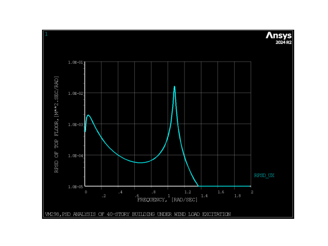
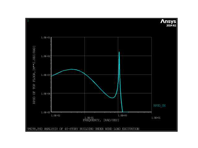
# The frequency distribution of the displacement response PSD at the top floor X_40
# is shown in the following figure. It is typical of wind response of tall structures.
# The first peak occurring around 0.04 rad/sec is due to the maximum of the wind spectrum
# (quasi-static response). The second peak occurring around 1.08 rad/sec coincides with
# the first natural frequency of the building (dynamic response).

mapdl.plvar(nvar1="5")

mapdl.screenshot()
mapdl.show("CLOSE")

Post-process PSD response plot using Matplotlib

ndim = len(mapdl.parameters["RPSD_UX"])

# store MAPDL results to python variables
mapdl.dim("frequencies", "array", ndim, 1)
frequencies = mapdl.vget("frequencies(1)", 4)

# store MAPDL results to python variables
mapdl.dim("response", "array", ndim, 1)
response = mapdl.vget("response(1)", 5)

# use Matplotlib to create graph
fig = plt.figure()
ax = fig.add_subplot(111)
# plt.xscale("log")
plt.yscale("log")
plt.ylim(1e-5, 1e-1)
plt.xlim(1e-2, 2)
ax.plot(frequencies, response)
ax.set_xlabel("FREQUENCY, [RAD/SEC]")
ax.set_ylabel("RPSD OF TOP FLOOR,[M**2.SEC/RAD]")
fig.show()

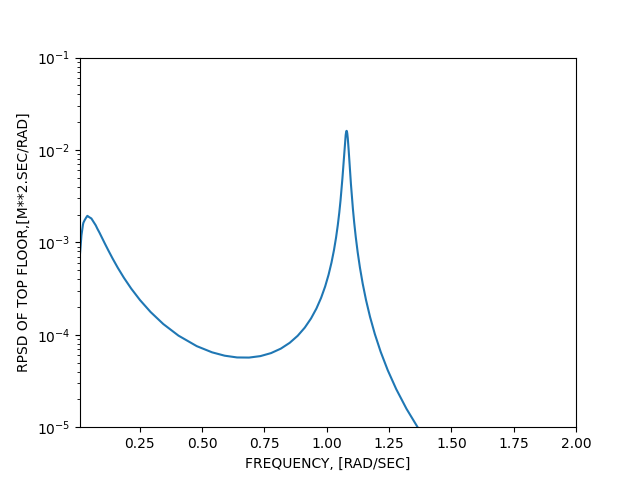
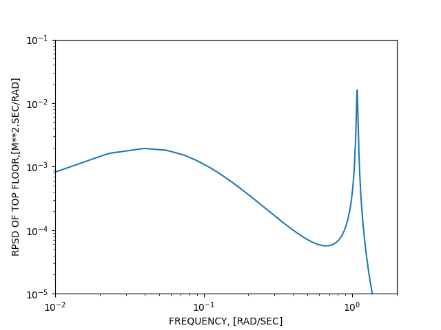
The above figure is plotted using lin-log scale to match Figure 2 in the reference. To better show the general shape of the response PSD, it is plotted using a log-log scale in the figure below.

Both plots are not the default response PSD (1-sided with m^2/Hz units). APDL operations are done on the results to obtain the 2-sided response PSD expressed in m^2/rad/s as is presented in the reference article.

Post-process PSD response using Matplotlib - Log-Log Scale

# PLOT RPSD LOG-LOG
mapdl.show("PNG", "REV")
mapdl.axlab("X", "FREQUENCY, [RAD/SEC]")
mapdl.axlab("Y", "RPSD OF TOP FLOOR,[M**2.SEC/RAD]")
mapdl.xrange(xmin="1E-2", xmax="2")
mapdl.gropt(lab="LOGX", key="ON")

mapdl.plvar(nvar1="5")

mapdl.screenshot()
mapdl.show("CLOSE")

Use Matplotlib to create graph

fig = plt.figure()
ax = fig.add_subplot(111)
plt.xscale("log")
plt.yscale("log")
plt.ylim(1e-5, 1e-1)
plt.xlim(1e-2, 2)
ax.plot(frequencies, response)
ax.set_xlabel("FREQUENCY, [RAD/SEC]")
ax.set_ylabel("RPSD OF TOP FLOOR,[M**2.SEC/RAD]")
plt.show()

Compute the standard deviation of the response PSD

# 1-SIGMA DISPLACEMENT SOLUTION FROM POST26 (RPSD INTEGRATION)
mapdl.int1(ir="6", iy="3", ix="1")

# VARIANCE
d_variance = mapdl.get(
    par="D_VARIANCE", entity="VARI", entnum="6", item1="EXTREME", it1num="VLAST"
)

# STANDARD DEVIATION
rms_value = math.sqrt(d_variance)

# REFERENCE STANDARD DEVIATION VALUE, SigmaX40 = 4.65E-2 M
print(f"rms_value={rms_value:0.2f}")

mapdl.finish()

rms_value=0.04

***** ROUTINE COMPLETED *****  CP =         0.000

Verify the results

from tabulate import tabulate

# Set target values
target_freq = 1.02
target_rms = 0.0465

# Fill result values
sim_freq_res = OMG_1
sim_rms_res = rms_value


# Using the computed displacement response PSD, the standard deviation is computed
# by integration and square root operations. It matches the 1-sigma displacement
# obtained directly in POST1 at load step 3 - substep 1. It is compared with the
# reference in the table below.

headers = ["Units", "TARGET", "Mechanical APDL", "RATIO"]
data_freq = [
    [
        "FREQ (rad/sec)",
        target_freq,
        sim_freq_res,
        np.abs(sim_freq_res) / np.abs(target_freq),
    ]
]
data_rms = [
    ["RMS Value (m)", target_rms, sim_rms_res, np.abs(sim_rms_res) / np.abs(target_rms)]
]

print(
    f"""
------------------- VM298 RESULTS COMPARISON ---------------------
MODAL FREQUENCY

{tabulate(data_freq, headers=headers)}

STANDARD DEVIATION OF RESPONSE PSD

{tabulate(data_rms, headers=headers)}

"""
)

------------------- VM298 RESULTS COMPARISON ---------------------
MODAL FREQUENCY

Units             TARGET    Mechanical APDL    RATIO
--------------  --------  -----------------  -------
FREQ (rad/sec)      1.02             1.0798  1.05863

STANDARD DEVIATION OF RESPONSE PSD

Units            TARGET    Mechanical APDL     RATIO
-------------  --------  -----------------  --------
RMS Value (m)    0.0465          0.0404041  0.868906

Stop MAPDL.

mapdl.exit()

""

''