Note
Go to the end to download the full example code.
Nuclear regulatory commission piping benchmarks#
- Problem description:
The example problem contains Mechanical APDL solutions to Nuclear Regulatory Commission (NRC) piping benchmark problems taken from publications NUREG/CR-1677, Volumes 1, Problem 1.
The piping benchmark solutions given in NRC publications were obtained by using a computer program EPIPE which is a modification of the widely available program SAP IV specifically prepared to perform piping analyses.
This benchmark problem contains three straight sections, two bends, and two fixed anchors. The total mass of the system is represented by structural mass element (MASS21) specified at individual nodes.
Modal and response spectrum analysis is performed on the piping model. Frequencies obtained from modal solve and the nodal/element solution obtained from spectrum solve are compared against reference results.
For response spectrum analysis, acceleration response spectrum curve defined by
SVandFREQcommands.
- Reference:
P.Bezler, M. Hartzman & M. Reich,”Dynamic Analysis of Uniform Support Motion Response Spectrum Method”, (NUREG/CR-1677), Brookhaven National Laboratory, August 1980, Problem 1, Pages 24-47.
- Analysis type(s):
Modal Analysis
ANTYPE=2Spectral Analysis
ANTYPE=8
- Element type(s):
Structural Mass Element (
MASS21)3-D 3-Node Pipe Element (
PIPE289)3-D 3-Node Elbow Element (
ELBOW290)
- Model description:
The model consists of a piping system with straight pipes and elbows.
The system is subjected to uniform support motion in three spatial directions.
The model is meshed using
PIPE289andELBOW290elements for the piping components andMASS21elements for point mass representation.
- Postprocessing:
Frequencies obtained from modal solution.
Maximum nodal displacements and rotations are extracted.
Element forces and moments are calculated for specific elements.
Reaction forces from the spectrum solution are obtained.
# sphinx_gallery_thumbnail_path = '_static/vm-nr1677-01-1a_setup.png'

""
# Import the MAPDL module
from ansys.mapdl.core import launch_mapdl
import numpy as np
from tabulate import tabulate

# Launch MAPDL with a specific log level and print command output
# Here, we set loglevel to "WARNING" to reduce verbosity and print_com to True to see commands
mapdl = launch_mapdl(loglevel="WARNING", print_com=True)

"""
Preprocessing: modeling of NRC piping benchmark problems using ``PIPE289`` and ``ELBOW290`` elements
-----------------------------------------------------------------------------------------------------

"""
'\nPreprocessing: modeling of NRC piping benchmark problems using ``PIPE289`` and ``ELBOW290`` elements\n-----------------------------------------------------------------------------------------------------\n\n'
Specify material properties, real constants and Element types
# Clear any previous data in MAPDL

mapdl.clear()

mapdl.title("NRC Piping Benchmark Problems, Volume 1, Problem 1")

mapdl.prep7(mute=True)

# Define Material Properties for pipe elements in :math:``psi``

mapdl.mp("ex", 1, 24e6)
mapdl.mp("nuxy", 1, 0.3)

# PIPE289 using cubic shape function and Thick pipe theory.

mapdl.et(1, "pipe289")
mapdl.keyopt(1, 4, 2)

# ELBOW290 using cubic shape function and number of Fourier terms = 6.

mapdl.et(2, "elbow290", "", 6)

# Real Constants for straight and bend pipe elements in :math:``in``

mapdl.sectype(1, "pipe")
mapdl.secdata(7.289, 0.241, 24)

# MASS21, 3-D Mass without Rotary Inertia

mapdl.et(3, "mass21")
mapdl.keyopt(3, 3, 2)

# Define real constants for mass elements, 3-D mass in :math:``lb-sec^2/in``

mapdl.r(12, 0.03988)  # Mass @ node 2
mapdl.r(13, 0.05032)  # Mass @ node 6
mapdl.r(14, 0.02088)  # Mass @ node 28
mapdl.r(15, 0.01698)  # Mass @ node 10
mapdl.r(16, 0.01307)  # Mass @ node 11
mapdl.r(17, 0.01698)  # Mass @ node 15
mapdl.r(18, 0.01044)  # Mass @ node 35
mapdl.r(19, 0.01795)  # Mass @ node 19
mapdl.r(20, 0.01501)  # Mass @ node 20
REAL CONSTANT SET         20  ITEMS   1 TO   6
   0.15010E-01   0.0000       0.0000       0.0000       0.0000       0.0000
Geometry modeling of nuclear piping system
# Define Keypoints

mapdl.k(1, 0.0, 0.0, 0.0)
mapdl.k(2, 0.0, 54.45, 0.0)
mapdl.k(3, 0.0, 108.9, 0.0)
mapdl.k(4, 10.632, 134.568, 0.0)
mapdl.k(5, 36.3, 145.2, 0.0)
mapdl.k(6, 54.15, 145.2, 0.0)
mapdl.k(7, 72.0, 145.2, 0.0)
mapdl.k(8, 97.668, 145.2, 10.632)
mapdl.k(9, 108.3, 145.2, 36.3)
mapdl.k(10, 108.3, 145.2, 56.80)
mapdl.k(11, 108.3, 145.2, 77.3)

mapdl.k(12, 2.7631, 122.79, 0)
mapdl.k(13, 22.408, 142.44, 0)
mapdl.k(14, 85.9, 145, 2.76)
mapdl.k(15, 106, 145, 22.4)

# Straight Pipe system

mapdl.l(1, 2)
mapdl.l(2, 3)
mapdl.l(5, 6)
mapdl.l(6, 7)
mapdl.l(9, 10)
mapdl.l(10, 11)  # Line number 6

# Bend Pipe system

mapdl.larc(3, 4, 12)  # Line number 7
mapdl.larc(4, 5, 13)
mapdl.larc(7, 8, 14)
mapdl.larc(8, 9, 15)  # line number 10
10
Meshing of nuclear piping system using pipe and elbow elements
# Meshing for straight pipe using PIPE289 elements

mapdl.type(1)
mapdl.mat(1)
mapdl.secnum(1)
mapdl.real(1)

mapdl.lsel("s", "line", "", 1, 6)
mapdl.allsel("below", "line")
mapdl.lesize("all", "", "", 2)
mapdl.lmesh("all")
mapdl.allsel("all", "all")

# Meshing for bend pipe using ELBOW290 elements

mapdl.type(2)
mapdl.secnum(1)
mapdl.mat(1)

mapdl.lsel("s", "", "", 7, 14)
mapdl.allsel("below", "line")
mapdl.lesize("all", "", "", 2)
mapdl.lmesh("all")
mapdl.allsel("all", "all")
SELECT ALL ENTITIES OF TYPE= ALL AND BELOW
The total system mass of nuclear piping system is represented by structural
mass element MASS21 specified at individual nodes.
# Specify mass elements with real constants at respective nodes

mapdl.type(3)
mapdl.real(12)
mapdl.e(2)  # Mass element at node 2

mapdl.real(13)
mapdl.e(6)  # Mass element at node 6

mapdl.real(14)
mapdl.e(28)  # Mass element at node 28

mapdl.real(15)
mapdl.e(10)  # Mass element at node 10

mapdl.real(16)
mapdl.e(11)  # Mass element at node 11

mapdl.real(17)
mapdl.e(15)  # Mass element at node 15

mapdl.real(18)
mapdl.e(35)  # Mass element at node 35

mapdl.real(19)
mapdl.e(19)  # Mass element at node 19

mapdl.real(20)
mapdl.e(20)  # Mass element at node 20
29
Using ELBOW, to convert some PIPE289 into ELBOW290
mapdl.elbow("on", "", "", "sect")
mapdl.allsel("all", "all")
SELECT ALL ENTITIES OF TYPE= ALL AND BELOW
Display the nuclear piping system model
mapdl.eplot()
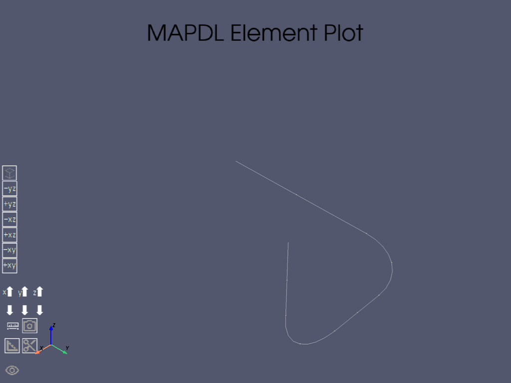
[82, 87, 110]
Define constraints
mapdl.dk(1, "all", 0)
mapdl.dk(11, "all", 0)
mapdl.allsel("all", "all")
SELECT ALL ENTITIES OF TYPE= ALL AND BELOW
Finish preprocessing aspects of nuclear piping system.
mapdl.finish()
***** ROUTINE COMPLETED ***** CP = 0.000
Modal analysis#
Perform modal analysis to obtain the first five natural frequencies of the system. The results will be used to determine the response spectrum analysis. The modal analysis is performed using the LANB method.
EXPAND ALL EXTRACTED MODES
  CALCULATE ELEMENT RESULTS AND NODAL DOF SOLUTION
Solve the modal analysis#
mapdl.solve()
mapdl.finish()
FINISH SOLUTION PROCESSING


 ***** ROUTINE COMPLETED *****  CP =         0.000
Postprocessing: Extracting frequencies from the modal analysis#
Frequencies from Modal solve:
 - 28.515 Hz
 - 56.441 Hz
 - 82.947 Hz
 - 144.139 Hz
 - 166.264 Hz

EXIT THE MAPDL POST1 DATABASE PROCESSOR


 ***** ROUTINE COMPLETED *****  CP =         0.000
Response spectrum analysis#
Perform spectrum analysis using the frequencies obtained from the modal analysis. The response spectrum analysis will be performed for a single point excitation response spectrum. The damping ratio is set to a constant value for all modes. The modes are grouped based on a significance level, and the seismic acceleration response loading is defined. The excitation is applied along the X, Y, and Z directions with specified frequencies and corresponding spectral values. Start the solution controls for spectrum solve
mapdl.slashsolu()

# Perform Spectrum Analysis
mapdl.antype("spectr")

# Single Point Excitation Response Spectrum
mapdl.spopt("sprs")

# specify constant damping ratio for all modes
mapdl.dmprat(0.02)

# Group Modes based on significance level
mapdl.grp(0.001)

# Seismic Acceleration Response Loading
mapdl.svtyp(2)
SPECTRUM TYPE KEY= 2 FACTOR= 1.00000
Solve the spectrum analysis along X direction#
Excitation along X direction
mapdl.sed(1)

mapdl.freq()  # Erase frequency values

mapdl.freq(3.1, 4, 5, 5.81, 7.1, 8.77, 10.99, 14.08, 17.24)
mapdl.freq(25, 28.5, 30, 34.97, 55, 80, 140, 162, 588.93)
mapdl.sv(0.02, 400, 871, 871, 700, 1188, 1188, 440, 775, 775)
mapdl.sv(0.02, 533.2, 467.2, 443.6, 380, 289, 239.4, 192.6, 184.1, 145)

mapdl.solve()
*****  MAPDL SOLVE    COMMAND  *****

 *** SELECTION OF ELEMENT TECHNOLOGIES FOR APPLICABLE ELEMENTS ***
                ---GIVE SUGGESTIONS ONLY---

 ELEMENT TYPE         1 IS PIPE289 . KEYOPT(4) IS ALREADY SET AS SUGGESTED FOR THICK-WALLED PIPES.

 ELEMENT TYPE         1 IS PIPE289 . KEYOPT(15) IS ALREADY SET AS SUGGESTED.


   *****MAPDL VERIFICATION RUN ONLY*****
     DO NOT USE RESULTS FOR PRODUCTION

                       S O L U T I O N   O P T I O N S

   PROBLEM DIMENSIONALITY. . . . . . . . . . . . .3-D
   DEGREES OF FREEDOM. . . . . . UX   UY   UZ   ROTX ROTY ROTZ
   ANALYSIS TYPE . . . . . . . . . . . . . . . . .SPECTRUM
      SPECTRUM TYPE. . . . . . . . . . . . . . . .SINGLE POINT
   GLOBALLY ASSEMBLED MATRIX . . . . . . . . . . .SYMMETRIC

                      L O A D   S T E P   O P T I O N S

   LOAD STEP NUMBER. . . . . . . . . . . . . . . .     1
   MODAL DAMPING RATIO . . . . . . . . . . . . . . 0.20000E-01
   SPECTRUM LOADING TYPE . . . . . . . . . . . . .ACCELERATION
   EXCITATION DIRECTION. . . . . . .  1.0000      0.0000      0.0000
   MODE COMBINATION TYPE . . . . . . . . . . . . . GRP
   RESPONSE TYPE . . . . . . . . . . . . . . . . .DISPLACEMENT
   SIGNIFICANCE LEVEL FOR COMBINATIONS. . . . . 0.10000E-02
   PRINT OUTPUT CONTROLS . . . . . . . . . . . . .NO PRINTOUT
   DATABASE OUTPUT CONTROLS. . . . . . . . . . . .ALL DATA WRITTEN

   *****MAPDL VERIFICATION RUN ONLY*****
     DO NOT USE RESULTS FOR PRODUCTION


            ***** RESPONSE SPECTRUM CALCULATION SUMMARY ******
                                                                                                            CUMULATIVE
 MODE      FREQUENCY        SV        PARTIC.FACTOR      MODE COEF.     M.C. RATIO    EFFECTIVE MASS      MASS FRACTION

     1       28.51      466.95         -0.1746         -0.2540E-02      1.000000       0.304998E-01          0.169869
     2       56.44      285.27          0.3636          0.8248E-03      0.324661       0.132216              0.906249
     3       82.95      236.06          0.5699E-01      0.4953E-04      0.019495       0.324763E-02          0.924337
     4       144.1      190.87          0.8193E-01      0.1907E-04      0.007505       0.671241E-02          0.961722
     5       166.3      183.22          0.8290E-01      0.1392E-04      0.005478       0.687280E-02           1.00000
                                                            SUM OF EFFECTIVE MASSES=  0.179549
   *****MAPDL VERIFICATION RUN ONLY*****
     DO NOT USE RESULTS FOR PRODUCTION

   SIGNIFICANCE FACTOR FOR COMBINING MODES = 0.10000E-02


     SIGNIFICANT MODE COEFFICIENTS (INCLUDING DAMPING)

 MODE     FREQUENCY    DAMPING       SV           MODE COEF.

    1       28.51         0.0200  466.95         -0.2540E-02
    2       56.44         0.0200  285.27          0.8248E-03
    3       82.95         0.0200  236.06          0.4953E-04
    4       144.1         0.0200  190.87          0.1907E-04
    5       166.3         0.0200  183.22          0.1392E-04

                    MODAL COMBINATION COEFFICIENTS

           MODE=   1  FREQUENCY=      28.515  COUPLING COEF.=   1.000
           MODE=   2  FREQUENCY=      56.441  COUPLING COEF.=   1.000
           MODE=   3  FREQUENCY=      82.947  COUPLING COEF.=   1.000
           MODE=   4  FREQUENCY=     144.139  COUPLING COEF.=   1.000
           MODE=   5  FREQUENCY=     166.264  COUPLING COEF.=   1.000

 GROUPING COMBINATION INSTRUCTIONS WRITTEN ON FILE file.mcom
Solve the spectrum analysis along Y direction#
Excitation along Y direction
mapdl.sed("", 1)

mapdl.freq()  # Erase frequency values

mapdl.freq(3.1, 4, 5, 5.81, 7.1, 8.77, 10.99, 14.08, 17.24)
mapdl.freq(25, 28.5, 30, 34.97, 55, 80, 140, 162, 588.93)
mapdl.sv(0.02, 266.7, 580.7, 580.7, 466.7, 792, 792, 293.3, 516.7, 516.7)
mapdl.sv(0.02, 355.5, 311.5, 295.7, 253.3, 192.7, 159.6, 128.4, 122.7, 96.7)

mapdl.solve()
*****  MAPDL SOLVE    COMMAND  *****
   *****MAPDL VERIFICATION RUN ONLY*****
     DO NOT USE RESULTS FOR PRODUCTION

                      L O A D   S T E P   O P T I O N S

   LOAD STEP NUMBER. . . . . . . . . . . . . . . .     2
   MODAL DAMPING RATIO . . . . . . . . . . . . . . 0.20000E-01
   SPECTRUM LOADING TYPE . . . . . . . . . . . . .ACCELERATION
   EXCITATION DIRECTION. . . . . . .  0.0000      1.0000      0.0000
   MODE COMBINATION TYPE . . . . . . . . . . . . . GRP
   RESPONSE TYPE . . . . . . . . . . . . . . . . .DISPLACEMENT
   SIGNIFICANCE LEVEL FOR COMBINATIONS. . . . . 0.10000E-02
   PRINT OUTPUT CONTROLS . . . . . . . . . . . . .NO PRINTOUT
   DATABASE OUTPUT CONTROLS. . . . . . . . . . . .ALL DATA WRITTEN

   *****MAPDL VERIFICATION RUN ONLY*****
     DO NOT USE RESULTS FOR PRODUCTION


            ***** RESPONSE SPECTRUM CALCULATION SUMMARY ******
                                                                                                            CUMULATIVE
 MODE      FREQUENCY        SV        PARTIC.FACTOR      MODE COEF.     M.C. RATIO    EFFECTIVE MASS      MASS FRACTION

     1       28.51      311.33          0.2673E-01      0.2592E-03      1.000000       0.714466E-03          0.958915E-02
     2       56.44      190.21         -0.3996E-02     -0.6044E-05      0.023312       0.159673E-04          0.980346E-02
     3       82.95      157.37          0.2584          0.1497E-03      0.577409       0.667536E-01          0.905733
     4       144.1      127.24         -0.5180E-01     -0.8035E-05      0.030995       0.268293E-02          0.941742
     5       166.3      122.11         -0.6588E-01     -0.7372E-05      0.028436       0.434068E-02           1.00000
                                                            SUM OF EFFECTIVE MASSES=  0.745077E-01
   *****MAPDL VERIFICATION RUN ONLY*****
     DO NOT USE RESULTS FOR PRODUCTION

   SIGNIFICANCE FACTOR FOR COMBINING MODES = 0.10000E-02


     SIGNIFICANT MODE COEFFICIENTS (INCLUDING DAMPING)

 MODE     FREQUENCY    DAMPING       SV           MODE COEF.

    1       28.51         0.0200  311.33          0.2592E-03
    2       56.44         0.0200  190.21         -0.6044E-05
    3       82.95         0.0200  157.37          0.1497E-03
    4       144.1         0.0200  127.24         -0.8035E-05
    5       166.3         0.0200  122.11         -0.7372E-05

                    MODAL COMBINATION COEFFICIENTS

           MODE=   1  FREQUENCY=      28.515  COUPLING COEF.=   1.000
           MODE=   2  FREQUENCY=      56.441  COUPLING COEF.=   1.000
           MODE=   3  FREQUENCY=      82.947  COUPLING COEF.=   1.000
           MODE=   4  FREQUENCY=     144.139  COUPLING COEF.=   1.000
           MODE=   5  FREQUENCY=     166.264  COUPLING COEF.=   1.000

 GROUPING COMBINATION INSTRUCTIONS WRITTEN ON FILE file.mcom
Solve the spectrum analysis along Z direction#
# Excitation along Z direction

mapdl.sed("", "", 1)

mapdl.freq()  # Erase frequency values

mapdl.freq(3.1, 4, 5, 5.81, 7.1, 8.77, 10.99, 14.08, 17.24)
mapdl.freq(25, 28.5, 30, 34.97, 55, 80, 140, 162, 588.93)
mapdl.sv(0.02, 400, 871, 871, 700, 1188, 1188, 440, 775, 775)
mapdl.sv(0.02, 533.2, 467.2, 443.6, 380, 289, 239.4, 192.6, 184.1, 145)

mapdl.solve()
*****  MAPDL SOLVE    COMMAND  *****
   *****MAPDL VERIFICATION RUN ONLY*****
     DO NOT USE RESULTS FOR PRODUCTION

                      L O A D   S T E P   O P T I O N S

   LOAD STEP NUMBER. . . . . . . . . . . . . . . .     3
   MODAL DAMPING RATIO . . . . . . . . . . . . . . 0.20000E-01
   SPECTRUM LOADING TYPE . . . . . . . . . . . . .ACCELERATION
   EXCITATION DIRECTION. . . . . . .  0.0000      0.0000      1.0000
   MODE COMBINATION TYPE . . . . . . . . . . . . . GRP
   RESPONSE TYPE . . . . . . . . . . . . . . . . .DISPLACEMENT
   SIGNIFICANCE LEVEL FOR COMBINATIONS. . . . . 0.10000E-02
   PRINT OUTPUT CONTROLS . . . . . . . . . . . . .NO PRINTOUT
   DATABASE OUTPUT CONTROLS. . . . . . . . . . . .ALL DATA WRITTEN

   *****MAPDL VERIFICATION RUN ONLY*****
     DO NOT USE RESULTS FOR PRODUCTION


            ***** RESPONSE SPECTRUM CALCULATION SUMMARY ******
                                                                                                            CUMULATIVE
 MODE      FREQUENCY        SV        PARTIC.FACTOR      MODE COEF.     M.C. RATIO    EFFECTIVE MASS      MASS FRACTION

     1       28.51      466.95          0.3311          0.4816E-02      1.000000       0.109602              0.825688
     2       56.44      285.27          0.1482          0.3361E-03      0.069798       0.219598E-01          0.991123
     3       82.95      236.06         -0.2864E-01     -0.2489E-04      0.005168       0.820073E-03          0.997301
     4       144.1      190.87         -0.1526E-01     -0.3552E-05      0.000738       0.232945E-03          0.999056
     5       166.3      183.22          0.1120E-01      0.1880E-05      0.000390       0.125338E-03           1.00000
                                                            SUM OF EFFECTIVE MASSES=  0.132740
   *****MAPDL VERIFICATION RUN ONLY*****
     DO NOT USE RESULTS FOR PRODUCTION

   SIGNIFICANCE FACTOR FOR COMBINING MODES = 0.10000E-02


     SIGNIFICANT MODE COEFFICIENTS (INCLUDING DAMPING)

 MODE     FREQUENCY    DAMPING       SV           MODE COEF.

    1       28.51         0.0200  466.95          0.4816E-02
    2       56.44         0.0200  285.27          0.3361E-03
    3       82.95         0.0200  236.06         -0.2489E-04

                    MODAL COMBINATION COEFFICIENTS

           MODE=   1  FREQUENCY=      28.515  COUPLING COEF.=   1.000
           MODE=   2  FREQUENCY=      56.441  COUPLING COEF.=   1.000
           MODE=   3  FREQUENCY=      82.947  COUPLING COEF.=   1.000

 GROUPING COMBINATION INSTRUCTIONS WRITTEN ON FILE file.mcom
Finish the spectrum analysis
mapdl.finish()
FINISH SOLUTION PROCESSING


 ***** ROUTINE COMPLETED *****  CP =         0.000
Postprocessing: extracting results from the spectrum analysis#
Extract maximum nodal displacements and rotations from the spectrum solution. The results will be stored in the MAPDL database and can be accessed using the starstatus command. The nodal displacements and rotations are obtained for specific nodes in the model. The element forces and moments are obtained for specific nodes from spectrum solution. The reaction forces from the spectrum solution are also extracted.
mapdl.post1()

mcom_file = mapdl.input("", "mcom")

adisx = mapdl.get("AdisX", "NODE", 10, "U", "X")
adisy = mapdl.get("AdisY", "NODE", 36, "U", "Y")
adisz = mapdl.get("AdisZ", "NODE", 28, "U", "Z")
arotx = mapdl.get("ArotX", "NODE", 9, "ROT", "X")
aroty = mapdl.get("ArotY", "NODE", 18, "ROT", "Y")
arotz = mapdl.get("ArotZ", "NODE", 9, "ROT", "Z")
Element Forces and Moments obtained from spectrum solution for Node “I”
elems = [12, 14]

# Output labels
# px = section axial force at node I and J.
# vy = section shear forces along Y direction at node I and J.
# vz = section shear forces along Z direction at node I and J.
# tx = section torsional moment at node I and J
# my = section bending moments along Y direction at node I and J.
# mz = section bending moments along Z direction at node I and J.
labels = ["px", "vy", "vz", "tx", "my", "mz"]

# SMISC mapping
# To obtain the SMISC values for each element
SMISC = {
    # Element number 12
    12: {
        # Obtained from the Element reference for PIPE289
        "i": [1, 6, 5, 4, 2, 3],
        "j": [14, 19, 18, 17, 15, 16],
    },
    # Element number 14
    14: {
        # Obtained from the Element reference for ELBOW290
        "i": [1, 6, 5, 4, 2, 3],
        "j": [36, 41, 40, 39, 37, 38],
    },
}

for elem in elems:
    mapdl.esel("s", "elem", "", elem)

    for node in ["i", "j"]:
        for label, id_ in zip(labels, SMISC[elem][node]):
            label_ = f"{label}{node}_{elem}"
            mapdl.etable(label_, "smisc", id_)

mapdl.allsel("all")
mapdl.run("/GOPR")
PRINTOUT RESUMED BY /GOP
Reaction forces from spectrum solution
reaction_force = mapdl.prrsol()
Finish postprocessing of response spectrum analysis.
mapdl.finish()
EXIT THE MAPDL POST1 DATABASE PROCESSOR


 ***** ROUTINE COMPLETED *****  CP =         0.000
Results comparison#
Frequencies obtained from modal solution#
The results obtained from the modal solution are compared against target values. The target values are defined based on the reference results from the NRC publication.
# Set target values
target_freq = np.array([28.515, 56.441, 82.947, 144.140, 166.260])  # in Hz

# Fill result values
sim_freq_res = [freq[1] for freq in freq_list]

# Store ratio
value_ratio = []
for i in range(len(target_freq)):
    con = sim_freq_res[i] / target_freq[i]
    value_ratio.append(np.abs(con))

print("Frequencies Obtained Modal Solution \n")

# Prepare data for tabulation
data_freq = [
    [i + 1, target_freq[i], sim_freq_res[i], value_ratio[i]]
    for i in range(len(target_freq))
]

# Define headers
headers = ["Mode", "Target", "Mechanical APDL", "Ratio"]

# Print table
print(
    f"""------------------- VM-NR1677-01-1-a.1 RESULTS COMPARISON ---------------------
{tabulate(data_freq, headers=headers, tablefmt="grid")}
"""
)

""
# Set target values
target_res = np.array(
    [7.830e-03, 2.648e-03, 1.748e-02, 1.867e-04, 2.123e-04, 7.217e-05]
)

# Fill result values
# adisx, adisy, adisz, arotx, aroty, arotz = 7.8e-03, 2.6e-03, 1.75e-02, 1.9e-04, 2.1e-04, 7.2e-05
sim_res = np.array([adisx, adisy, adisz, arotx, aroty, arotz])

# Output labels
labels = [
    "UX at node10",
    "UY at node36",
    "UZ at node28",
    "ROTX at node9",
    "ROTY at node18",
    "ROTZ at node9",
]

# Store ratio
value_ratio = []
for i in range(len(target_res)):
    con = sim_res[i] / target_res[i]
    value_ratio.append(np.abs(con))

print("Maximum nodal displacements and rotations obtained from spectrum solution:")

# Prepare data for tabulation
data_freq = [
    [labels[i], target_res[i], sim_res[i], value_ratio[i]]
    for i in range(len(target_res))
]

# Define headers
headers = ["Result Node", "Target", "Mechanical APDL", "Ratio"]

# Print table
print(
    f"""
{tabulate(data_freq, headers=headers, tablefmt="grid")}
"""
)
Frequencies Obtained Modal Solution

------------------- VM-NR1677-01-1-a.1 RESULTS COMPARISON ---------------------
+--------+----------+-------------------+----------+
|   Mode |   Target |   Mechanical APDL |    Ratio |
+========+==========+===================+==========+
|      1 |   28.515 |           28.5149 | 0.999996 |
+--------+----------+-------------------+----------+
|      2 |   56.441 |           56.4409 | 0.999999 |
+--------+----------+-------------------+----------+
|      3 |   82.947 |           82.9473 | 1        |
+--------+----------+-------------------+----------+
|      4 |  144.14  |          144.139  | 0.999995 |
+--------+----------+-------------------+----------+
|      5 |  166.26  |          166.264  | 1.00002  |
+--------+----------+-------------------+----------+

Maximum nodal displacements and rotations obtained from spectrum solution:

+----------------+-----------+-------------------+---------+
| Result Node    |    Target |   Mechanical APDL |   Ratio |
+================+===========+===================+=========+
| UX at node10   | 0.00783   |       0.00783071  | 1.00009 |
+----------------+-----------+-------------------+---------+
| UY at node36   | 0.002648  |       0.00264813  | 1.00005 |
+----------------+-----------+-------------------+---------+
| UZ at node28   | 0.01748   |       0.0174804   | 1.00003 |
+----------------+-----------+-------------------+---------+
| ROTX at node9  | 0.0001867 |       0.000186769 | 1.00037 |
+----------------+-----------+-------------------+---------+
| ROTY at node18 | 0.0002123 |       0.000212341 | 1.00019 |
+----------------+-----------+-------------------+---------+
| ROTZ at node9  | 7.217e-05 |       7.21737e-05 | 1.00005 |
+----------------+-----------+-------------------+---------+
Element forces and moments obtained from spectrum solution for specific elements#
# For Node# 12:

# Set target values
TARGET = {
    12: {
        "i": np.array([24.019, 7.514, 34.728, 123.39, 2131.700, 722.790]),
        "j": np.array([24.018, 7.514, 34.728, 123.39, 2442.700, 786.730]),
    },
    14: {
        "i": np.array([5.1505, 7.2868, 7.9178, 450.42, 675.58, 314.970]),
        "j": np.array([6.006, 6.6138, 7.9146, 157.85, 858.09, 302.940]),
    },
}

sections = [
    "Axial force",
    "Shear force Y",
    "Shear force Z",
    "Torque",
    "Moment Y",
    "Moment Z",
]


for node, element in zip([12, 14], ["Pipe289", "Elbow290"]):
    print("\n\n===================================================")
    print(f"Element forces and moments at element {node} ({element})")
    print("===================================================")

    etab_i = [
        f"pxi_{node}",
        f"vyi_{node}",
        f"vzi_{node}",
        f"txi_{node}",
        f"myi_{node}",
        f"mzi_{node}",
    ]
    etab_j = [
        f"pxj_{node}",
        f"vyj_{node}",
        f"vzj_{node}",
        f"txj_{node}",
        f"myj_{node}",
        f"mzj_{node}",
    ]
    targets_i = TARGET[node]["i"]
    targets_j = TARGET[node]["j"]

    for each_section, each_tab_i, each_tab_j, target_i, target_j in zip(
        sections, etab_i, etab_j, targets_i, targets_j
    ):

        print(f"\n{each_section}")
        print("=" * len(each_section))

        # Element forces and moments at element, node "i"
        values_i = ["Node i"]

        values_i.append(mapdl.get_array("ELEM", "", "ETAB", each_tab_i)[node - 1])
        values_i.append(target_i)
        values_i.append(values_i[1] / target_i)

        # Element forces and moments at element , node "j"
        values_j = ["Node j"]

        values_j.append(mapdl.get_array("ELEM", "", "ETAB", each_tab_j)[node - 1])
        values_j.append(target_j)
        values_j.append(values_j[1] / target_j)

        headers = ["Node", "Mechanical APDL", "Target", "Ratio"]
        print(tabulate([values_i, values_j], headers=headers))
===================================================
Element forces and moments at element 12 (Pipe289)
===================================================

Axial force
===========
Node      Mechanical APDL    Target     Ratio
------  -----------------  --------  --------
Node i            24.0183    24.019  0.999972
Node j            24.0183    24.018  1.00001

Shear force Y
=============
Node      Mechanical APDL    Target    Ratio
------  -----------------  --------  -------
Node i            7.51454     7.514  1.00007
Node j            7.51454     7.514  1.00007

Shear force Z
=============
Node      Mechanical APDL    Target     Ratio
------  -----------------  --------  --------
Node i            34.7279    34.728  0.999996
Node j            34.7279    34.728  0.999996

Torque
======
Node      Mechanical APDL    Target    Ratio
------  -----------------  --------  -------
Node i            123.394    123.39  1.00003
Node j            123.394    123.39  1.00003

Moment Y
========
Node      Mechanical APDL    Target    Ratio
------  -----------------  --------  -------
Node i            2131.74    2131.7  1.00002
Node j            2442.7     2442.7  1

Moment Z
========
Node      Mechanical APDL    Target     Ratio
------  -----------------  --------  --------
Node i            722.787    722.79  0.999995
Node j            786.732    786.73  1


===================================================
Element forces and moments at element 14 (Elbow290)
===================================================

Axial force
===========
Node      Mechanical APDL    Target     Ratio
------  -----------------  --------  --------
Node i            5.15045    5.1505  0.999991
Node j            6.00561    6.006   0.999935

Shear force Y
=============
Node      Mechanical APDL    Target     Ratio
------  -----------------  --------  --------
Node i            7.29874    7.2868  1.00164
Node j            6.61379    6.6138  0.999999

Shear force Z
=============
Node      Mechanical APDL    Target     Ratio
------  -----------------  --------  --------
Node i            7.91776    7.9178  0.999995
Node j            7.91457    7.9146  0.999996

Torque
======
Node      Mechanical APDL    Target    Ratio
------  -----------------  --------  -------
Node i            450.42     450.42  1
Node j            157.852    157.85  1.00001

Moment Y
========
Node      Mechanical APDL    Target     Ratio
------  -----------------  --------  --------
Node i            675.577    675.58  0.999995
Node j            858.093    858.09  1

Moment Z
========
Node      Mechanical APDL    Target    Ratio
------  -----------------  --------  -------
Node i            314.972    314.97  1.00001
Node j            302.942    302.94  1.00001
Reaction forces#
Reaction forces
===============
  NODE      FX      FY      FZ       MX       MY       MZ
------  ------  ------  ------  -------  -------  -------
     1  17.93   4.9882  36.52   3231.9    648.47  1390.8
    24  34.728  7.5145  24.018   786.73  2442.7    123.39
Stop MAPDL#
mapdl.exit()
Total running time of the script: (0 minutes 1.593 seconds)